Tutorial on Bayesian hierarchical models

In this tutorial, we will motivate Bayesian hierarchical models and walk through a representative example showing how Bayesian hierarchical models are constructed. We will use a dataset of rocket launches to illustrate the concepts.

Application context

Hierachical modelling is a crown jewel of Bayesian statistics. Hierarchical modelling allows us to mitigate a common criticism against Bayesian models: sensitivity to the choice of prior distribution.

Prior sensitivity means that small differences in the choice of prior distribution (e.g. in the choice of the parameters of the prior distribution) will lead to large differences in posterior distributions. Prior sensitivity often arises when the size of the dataset is small. To examplify prior sensitivity, consider the task of predicting the success or failure of a future rocket launch. More precisely, we will consider prediction of the success/failure for the next launch of the Delta 7925H rocket, which as of November 2020 has been launched 3 times, with 0 failed launches. Maximum likelihood would therefore give an estimate of 0% for the chance of failure. Obviously we will not use this crazy estimate today and instead use Bayesian methods.

Let us start with the simplest Bayesian model for this task: we assume the three launches are independent, biased coin flips, all with a shared probability of failure (bias) given by an unknown parameter failureProbability. In other words, we assume a binomial likelihood. We also assume a beta prior on the failureProbability, the parameter $p$ of the binomial (the parameter $n$ is known and set to the number of observed launches, numberOfLaunches).

Let us walk over an implementation of this simple model in the Blang Probabilistic Programming Language:

Some explanations of the above code:

• The laws { ... } block specifies a joint distribution over a collection of random variables, namely those marked with the keyword random when they are declared above. Each line starting in the form variable ~ ... declares a distribution or conditional distribution.

• Each random variable can be either unobserved (like failureProbability here, marked using ?: latentReal) or observed (like numberOfFailures here, marked with an observed value via ?: 0). Running this Blang code will approximate the posterior distribution of the random variables that are unobserved given those that are observed.

• Click on "See output" above to see the main plots created by running the code. You can find in particular a visualization of the posterior distribution on the random variable failureProbability by following the tab "Plots" located in the top right of the page linked by "See output". The plot also shows a 90% credible interval in red.

Motivation: prior sensitivity

To motivate the need for hierarchical models, we will now use our rocket example to demonstrate that the posterior distribution is sensitive to the choice of prior when the dataset is small.

But before doing this, we will transform the parameters of the beta prior ($\alpha$ and $\beta$) into a new pair of parameters ($\mu$ and $s$) which are more interpretable. The transformation we use is:

$$\begin{align} \mu = \frac{\alpha}{\alpha + \beta}, \;\; s = \alpha + \beta \end{align}$$

where $\mu \in (0, 1)$, $s > 0$, which is invertible with an inverse given by

$$\begin{align} \alpha = \mu s, \;\; \beta = (1 - \mu) s. \end{align}$$

The interpretation of this reparameterization is:

• $\mu$: the mean of the prior distribution,

• $s$: a measure of "peakiness" of the prior density; higher $s$ correspond to a more peaked density; roughly, $s \approx$ number of data points ("pseudo-observations") that would make the posterior peaked like that.

Here is the reparameterized code, which gives the same approximation as before ($\mu$ is labelled mu in the code)

For reference, the Blang model for the reparameterized beta called by the above model is as follows:

Notice that instead of hard-coding the parameters of the prior, as we did in the first Blang model, in the model called BasicReparameterized shown earlier we migrated the prior parameters into command line arguments. This is achieved by defining two variables with the param keyword. We can now use a command line argument like --model.mu 0.1 to change the default value of $0.5$.

Side data

How to attenuate prior sensitivity? The key idea that will lead us to hierarchical models is to use side data to inform the prior. Back to the rocket application, recall that we are interested in one type of rocket called Delta 7925H. In this context, side data takes the form of success/fail launch data from other types of rockets.

Here is the data that we will use (showing only the first 10 rows out of 334 rows):

	rocketType	country	family	numberOfLaunches	numberOfFailures
1	Aerobee	USA	Aerobee	1	0
2	Angara A5	Russia/USSR	Angara	1	0
3	Antares 110	USA	Antares	2	0
4	Antares 120	USA	Antares	2	0
5	Antares 130	USA	Antares	1	1
6	Antares 230	USA	Antares	5	0
7	Antares 230+	USA	Antares	3	0
8	Ariane 1	Europe	Ariane	11	2
9	Ariane 2	Europe	Ariane	6	1
10	Ariane 3	Europe	Ariane	11	1
11	Ariane 40	Europe	Ariane	7	0

Can we use this side data to inform prediction for Delta 7925H launches?

Non-Bayesian use of side data

Before we describe the Bayesian way to use side data, let us briefly go over a more naive method. For now, let us focus on the prior parameter $\mu$.

Here is the naive method to determine the prior parameter $\mu$ from our "side data":

1. Estimate the failure probability $p_i$ for each rocket type $i$ (e.g. using maximum likelihood estimation, for binomial this is just the fraction of rocket failures for each rocket type). Let us denote each estimate by $\hat p_i$.

2. Fit a distribution over all the estimated failure probabilities $\hat p_i$'s

3. Use this fit distribution as the prior on $\mu$.

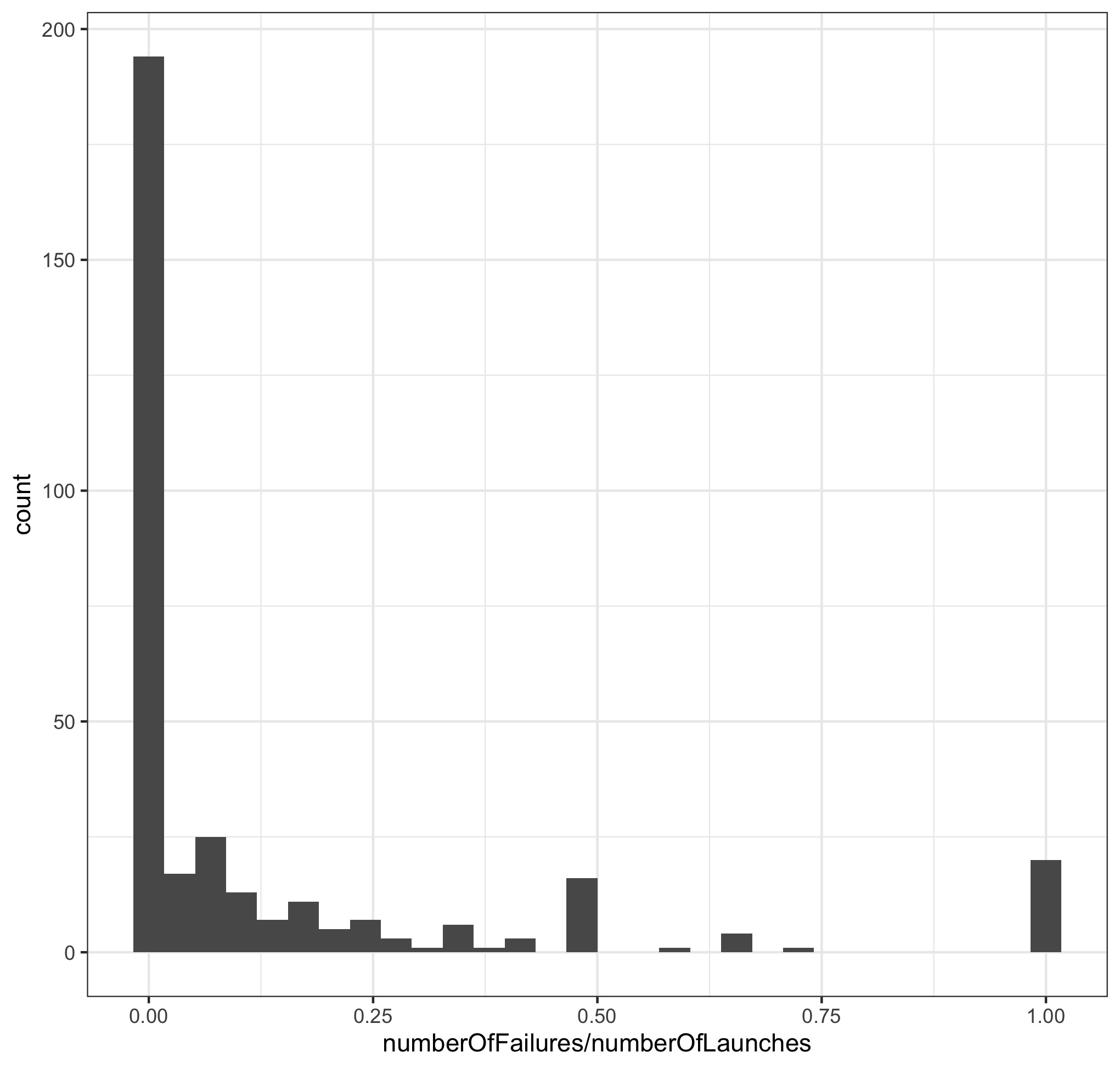
This method provides some intuition on how we can use side data to inform our choice of prior distribution. However this naive method has some weaknesses. A first weakness is that it is less obvious how to proceed with the precision parameter $s$. A second weakness is that the distribution estimated in step 2 above has some irregularities, visible in the histogram of MLE-estimated $\hat p_i$'s in our dataset

Bayesian use of side data

A general principle in Bayesian inference is to treat unknown quantities as random. This is also the essence of a Bayesian hierarchical model: let us treat $\mu$ and $s$ as random and let the side data inform their posterior distribution.

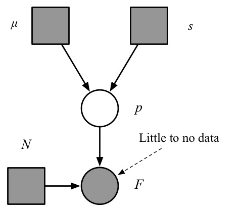
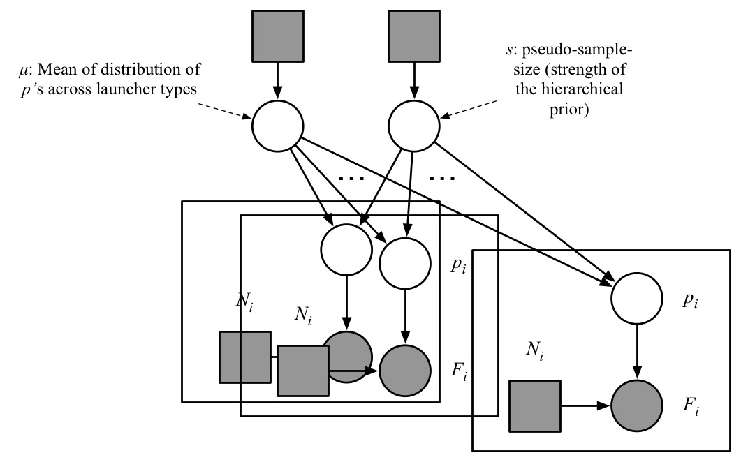
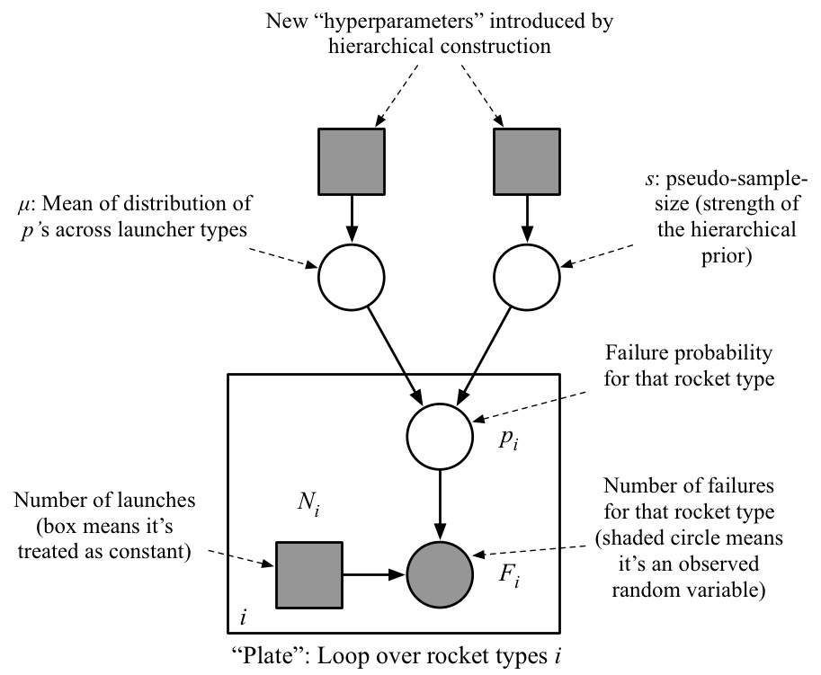
To visualize what a hierarchical model is, let us look at the corresponding graphical model, shown here. The circles are random variables, the squares, non-random. Shaded nodes are observed, white ones, unknown. An arrow from a variable $X$ to $Y$ means that the generative model for $Y$ has a parameter that depends on $X$. The rectangle enclosing the bottom three nodes is called a plate, encoding the fact that the "plated" random variables (those inside the rectangle) are copied, once for each rocket type (i.e. for each row in the data table shown earlier).

The model inside the plate is just several copies of the BasicReparameterized model. You can think of this as the "bottom level" of a hierarchy. What we have added in the hiearchical model is the "top level", which consists of two random variables, one for $\mu$, and one for $s$, each with its own prior distribution. Here we will use a beta prior for $\mu$ and an exponential prior for $s$.

Let us look at how to implement this model in Blang:

Some explanations of the above code:

• Variable of type Plate correspond to the plate rectangle shown earlier in the graphical model. A plate can be tought of as a collection of indices. The indices are automatically constructed by looking into the csv file (table above) for a column with a name (header) matching the name of the plate in the Blang file, here rocketType.

• Variables of type Plated correspond to a variable enclosed within a plate.

• GlobalDataSource is a mechanism to indicate that all plates and plated random variables will be extracted from a single csv file (with a path specified in the command line via --model.data data/rockets-2020/counts.csv.

Note that the new model still has prior distributions at the top level, and hence parameters to set for these new top level priors. Are we back to square one? No, as it turns out these top-level parameters will be generally less sensitive as you will verify in this exercise:

How to explain this reduced sensitivity? One heuristic is based on the graphical model. For each unobserved (white) node in the graphical model, the number of edges connected to that node is often indicative of how peaky the posterior distribution is, and peaky posteriors tend to be less sensitive to prior choice. Consider for example the graphical model for the basic model (left below). Note that the variable $p$ (failure probability for the Delta 7925H) has only 3 edges connected to it. Even if we expanded the observed number of failures ($F$) to a list of Bernoulli random variables, this would only lead to two more connections. In contrast, with the hierarchical model (right), the top nodes have 334 connections (the number of rocket types, i.e. rows in the data table). The theorem behind this vague heuristic is the Bernstein–von Mises theorem.