Instructor: Alexandre Bouchard-Côté
Editor: Neil Spencer

Based on: lecture 3,5 from last year.

More examples of losses

An example of loss for predicting a real number: squared loss

If you have not seen this material before, show that in the special case where $L$ is the squared loss on $L(a, z) = (z - a)^2$, one can compute a simple expression for the minimizer, which is simply $\delta^*(X) = \E[Z|X]$.

For other losses finding such an expression may or may not be possible. We will talk about approximation strategies for the latter case later in this course.

An example of loss for predicting the next point

In the case of density estimation, if the task is to reconstruct the density itself, a reasonable choice is to pick an intrinsic loss. Intrinsic loss functions are derived from sampling distributions based on the notion of "distances" between distributions. Such a loss functions are desirable because they have minimal influence on inference (the loss function analog to non-informative priors), and are not dependent on the parameterization of distributions.

Note that density estimation is usually an intermediate step for another task. In such cases the loss function should be defined on this final task rather than on the intermediate density estimation task. Otherwise, the intrinsic loss gives you a "default" choice of loss defined by computing distance of two distribution or densities (here the "action" is to pick one value for the latent z): \begin{eqnarray} L(z, z') = d(\ell(\cdot|z), \ell(\cdot|z')), \end{eqnarray} where $d$ is a distance or divergence between distributions.

The following are two examples of distances leading to intrinsic loss functions. Note that the Kullback-Leibler distance is much more commonly used due to its tractability and ties with information theory.

The Kullback-Leibler (KL) divergence:

\begin{eqnarray} L(z', Z) = \E \left[ \log\left( \frac{\ell(X|Z)}{\ell(X|z')} \right) | Z \right], \end{eqnarray}

where $Z$ can be interpreted at the true but unknown latent variable, and $Z'$ is our guess (action). Note that this is not symmetric in its arguments and not always defined (but if the support of all the likelihoods are the same it will be defined). On the other hand, it is invariant to the parameterization of the likelihood.

The Hellinger distance:

\begin{eqnarray} L(z', Z) = \frac{1}{2} \E \left[ \left( \sqrt{\frac{\ell(X|z')}{\ell(X|Z)}} - 1 \right)^2 | Z \right]. \end{eqnarray}

This always exists (bounded by one), it is symmetric (and a proper distance) and is also invariant to the parameterization of the likelihood.

Exercise: Suppose $X|Z$ is normally distributed with mean $Z$ and variance one, and we put a normal prior on $Z$. Find the Bayes estimator for the KL intrinsic loss.

Exercise (harder): Assume now that $X|Z$ is exponential with rate $Z$, and that the posterior was approximated by some MC samples $Z^{(1)}, \dots, Z^{(N)}$. How would you approach the problem of approximating the Bayes estimator for the Hellinger intrinsic loss in this case? Hint: the Hellinger distance is given by $1 - 2\sqrt{z'z}/(z' + z)$ in the exponential case.

More generally, can the Bayes estimator be approximated using MC samples for any "black box" loss (i.e. a loss where all you can do is do pointwise evaluation)? Can this be done in a computationally efficient manner (in the sense that the computational cost is not significantly more than it takes to run the MCMC chain)?

An example of loss for clustering: rand loss

In clustering analysis, the objective is to find a partition $\rho$ which divides the indices of the datapoints into "blocks" or "clusters". The points in the first cluster are explained using a first parametric model, the points in the second cluster are explained using a second parametric model, etc. Here we will focus on a loss function for clustering rather than the probabilistic model. We will come back to the probabilistic model for clustering next week.

Here, we discuss a popular loss function for clustering known as the rand loss. For true and putative labeled partitions $\rhot, \rhop$, the rand loss function is denotes as $\randindex(\rhot, \rhop)$. Note that we turn the standard notion of rand index into a loss by taking 1 - the rand index.

---

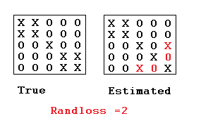
Definition: The rand loss is defined as the number of (unordered) pairs of data points indices ${i,j}$ such that $(i \sim_{\rhot} j) \neq (i \sim_{\rhop} j)$, i.e.: \begin{eqnarray} \sum_{1\le i < j \le n} \1[(i \sim_\rhot j) \neq (i \sim_\rhop j)], \end{eqnarray} where $(i \sim_\rho j) = 1$ if there is a $B\in\rho$ s.t. $\{i,j\}\subseteq B$, and $(i \sim_\rho j) = 0$ otherwise.

In other words, a loss of one is incurred each time either: (1) two points are assigned to the same cluster when they belong in separate clusters, or (2) two points are assigned to different clusters when they should be in the same cluster.

---

The rand loss has several problems, motivating other clustering losses such as the adjusted rand index, but we will look at the rand loss here since the derivation of the Bayes estimator is easy for that particular loss. (See Fritsch and Ickstadt, 2009 for discussion on other losses and how to approach the Bayes estimator optimization problem for these other losses.)

As reviewed earlier, the Bayesian framework is reductionist: given a loss function $L$ and a probability model $(\rho, X) \sim \P$, it prescribes the following estimator: \begin{eqnarray} \argmin_{\rho'} \E[L(\rho', \rho) | X]. \end{eqnarray}

We will now demonstrate, using the current example, how this abstract quantity can be computed or approximated in practice.

First, for the rand loss, we can write: \begin{eqnarray} \argmin_{\textrm{partition }\rho'} \E\left[\randindex(\rho, \rho')|X\right] & = & \argmin_{\textrm{partition }\rho'} \sum_{i<j} \E \left[\1 \left[\rho_{ij} \neq \rho'_{ij}\right]|X\right] \\ &=&\argmin_{\textrm{partition }\rho'} \sum_{i<j} \left\{(1-\rho'_{ij})\P(\rho_{ij} = 1|X) + \rho'_{ij} \left(1- \P(\rho_{ij} = 1 |X)\right)\right\} \label{eq:loss-id} \end{eqnarray} where $\rho_{i,j} = (i \sim_{\rho} j)$, which can be viewed as edge indicators on a graph.

The above identity comes from the fact that $\rho_{i,j}$ is either one or zero, so:

• the first term in the the brackets of Equation~(\ref{eq:loss-id}) corresponds to the edges not in the partition $\rho$ (for which we are penalized if the posterior probability of the edge is large), and
• the second term in the same brackets corresponds to the edges in the partition $\rho$ (for which we are penalized if the posterior probability of the edge is small).

This means that computing an optimal bipartition of the data into two clusters can be done in two steps:

1. Simulating a Markov chain, and use the samples to estimate $\partstrength_{i,j} = \P(\rho_{ij} = 1 | Y)$ via Monte Carlo averages.
2. Minimize the linear objective function $\sum_{i<j} \left\{(1-\rho_{ij})\partstrength_{i,j} + \rho_{ij} \left(1- \partstrength_{i,j}\right)\right\}$ over bipartitions $\rho$.

Note that the second step can be efficiently computed using min-flow/max-cut algorithms (understanding how this algorithm works is outside of the scope of this lecture, but if you are curious, see CLRS, chapter 26).

Consistency result for Bayesian statistics

Assumptions:

• We have a parametric model as described last time. $\ell(\cdot|z)$.
• The likelihood family is identifiable: $\P_z \neq \P_{z'}$ whenever $z \neq z'$.
• The prior $\Pi$ is positive on the space of unknown parameters $\Zscr$.

Notation:

• Let $\Pi(\cdot|x_{1:n})$ denote the posterior distribution obtained by seeing $n$ datapoints $x_{1:n}$. This distribution corresponds to the density $p(\cdot|x)$ from last time.
• Similarly let $\Pi$ denote the prior distribution,
• Let $\P_z$ denote the conditional distribution corresponding to the density $\ell(\cdot|z)$

Doob's consistency theorem: Under the above assumptions,

\begin{eqnarray} \P\left( \Pi(\cdot|X_{1:n}) \to \delta_Z(\cdot) \right) = 1, \end{eqnarray}

where $\delta$ denote the dirac distribution on the true parameter $Z$, and $\to$ denotes convergence in distribution. That is, $\mu_n \to \mu$ if for all continuous bounded $\phi$,

\begin{eqnarray} \int \phi (\tilde z) \mu_n(\ud \tilde z) \to \int \phi (\tilde z) \mu(\ud \tilde z). \end{eqnarray}

Notes:

• This result is extremely useful in practice for debugging.
• This result can break in non-parametric models.
• van der Vaart, p.149 provides a proof of this result. Asymptotic normality also holds under additional conditions.
• What if the prior $\Pi$ is very wrong (e.g. wrong support/structure)? Not much protection within the Bayesian framework for model mis-specification. Use frequentist validation! E.g.: cross validation, coverage assessment.

Well-specified Bayesian models exist, but can force us to be non-parametric

Let us make the discussion on de Finetti from last week more formal.

Recall: A finite sequence of random variables $(X_1, \dots, X_n)$ is exchangeable if for any permutation $\sigma : \{1, \dots, n\} \to \{1, \dots, n\}$, we have:

\begin{eqnarray} ({X_1}, \dots, {X_n}) \deq ({X_{\sigma(1)}}, \dots, {X_{\sigma(n)}}). \end{eqnarray}

Extension: A countably infinite sequence of random variable $(X_1, X_2, \dots)$ is (infinitely) exchangeable if all finite sub-sequence $(X_{k_1}, \dots, X_{k_n})$ are exchangeable.

Theorem: De Finetti (simple version): If $(X_1, X_2, \dots)$ is an exchangeable sequence of binary random variables, $X_i : \Omega' \to \{0,1\}$ then there exists a random variable $Z : \Omega' \to [0, 1]$ such that $X_i | Z \sim \Bern(Z)$.

In other words, if all we are modelling is a sequence of exchangeable binary random variables, we do not need a non-parametric model. On the other hand, if the $X_i$ are real, the situation is different:

Theorem: De Finetti (more general version, see Kallenberg, 2005, Chapter 1.1): If $(X_1, X_2, \dots)$ is an exchangeable sequence of real-valued random variables, the there exists a random measure $G : \Omega' \to (\sa_{\Omega} \to [0,1])$ such that $X_i | G \sim G$.

Supplementary references and notes

Robert, C. (2007) The Bayesian Choice. An excellent textbook, especially for the theoretically foundations of Bayesian statistics. Also covers many practical topics. Most relevant to this course are chapters 2, 3.1-3.3, 4.1-4.2.

van der Vaart, A.W. (1998) Asymptotic Statistics. Chapter 10 contains a formal treatment of the asymptotic properties of parametric Bayesian procedures. Note that a different treatment is needed for non-parametric Bayesian procedures.