Instructor: Alexandre Bouchard-Côté
Editor: Crystal Zhao

Prior choice and hierarchical models

We have touched on a first method to deal with prior hyper-parameters in this exercise. Here we discuss alternative methods.

Since conjugacy leads us to consider families of priors indexed by a hyper-parameter $h$, this begs the question of how to pick $h$. Note that both $m_h(x)$ and $p_h(z | x)$ implicitly depend on $h$. Here are some guidelines for approaching this question:

1. One can maximize $m_h(x)$ over $h$, an approach called empirical Bayes. Note however that this does not fit the Bayesian framework (despite its name). It estimate the hyperparameters from observations and the estimated prior is used in later analysis.
2. If the dataset is moderate to large, one can test a range of reasonable values for $h$ (a range obtained for example from discussion with a domain expert); if the action selected by the Bayes estimator is not affected (or not affected too much), one can side-step this issue and pick arbitrarily from the set of reasonable values.
3. If it is an option, one can collect more data from the same population. Under regularity conditions, the effect of the prior can be decreased arbitrarily (this follows from the celebrated Bernstein-von Mises theorem, see van der Vaart, p.140).
4. If we only have access to other datasets that are related (in the sense that they have the same type of latent space $\Zscr$), but potentially from different populations, we can still exploit them using a hierarchical Bayesian model, described next.

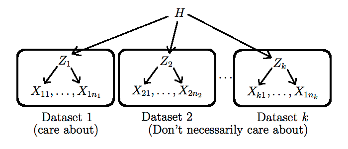
Hierarchical Bayesian models are conceptually simple:

1. We create distinct, exchangeable latent variables $Z_j$, one for each related dataset $X_j$
2. We make the hyper-parameter $h$ be the realization of a random variable $H$. This allows the dataset to originate from different populations.
3. We force all $Z_j$ to share this one hyper-parameter. This step is crucial as it allows information to flow between the datasets.

One still has to pick a new prior $p^*$ on $H$, and to go again through steps 1-4 above, but this time with more data incorporated. Note that this process can be iterated as long as there is some form of known hierarchical structure in the data (as a concrete example of a type of dataset that has this property, see this non-parametric Bayesian approach to $n$-gram modelling: Teh, 2006). More complicated techniques are needed when the hierarchical structure is unknown (we will talk about two of these techniques later in this course, namely hierarchical clustering and phylogenetics).

A formal definition of a Hierachical Bayesian model can be found in : Robert, C. (2007). You can also find some interesting examples of Hierachical Bayesian models in Chapter 10 of Robert, C. (2007). The assumption of exchangeability is often assumed in Hierarchical Bayesian Models.

Definition: A sequence of random variables $X_1, X_2,..., X_n$ is exchangeable if for any permutation $\sigma$ \begin{eqnarray} \sigma(1, ..., n) \rightarrow (1, ..., n) \\ (X_1, ..., X_n)\overset{d}{=} (X_{\sigma(1)}, ..., X_{\sigma(n)}). \end{eqnarray}

You can also find the difference amond finite exchangeability, infinite exchangeability and i.i.d at the wikipedia entry and entry for details.

The cost of taking the hierarchical Bayes route is that it generally requires resorting to Monte Carlo approximation, even if the initial model is conjugate.

Mixture models.

Example: Modelling the weight of walruses.

Observation: weights of specimens $x_1, x_2, ..., x_n$.

Inferential question: what is the most atypical weight among the samples?

Method 1:

• Find a normal density $\phi_{\mu, \sigma^2}$ that best fits the data.
• Bayesian way: treat the unknown quantity $\phi_{\mu, \sigma^2}$ as random.
• Equivalently: treat the parameters $\theta = (\mu, \sigma^2)$ as random, $(\sigma^2 > 0)$. Let us call the prior on this, $p(\theta)$ (for example, another normal times a gamma, but this will not be important in this first discussion).

Limitation: fails to model sexual dimorphism (e.g. male walruses are typically heavier than female walruses).

Solution: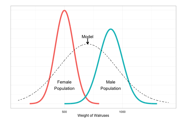

Method 2: Use a mixture model, with two mixture components, where each one assumed to be normal.

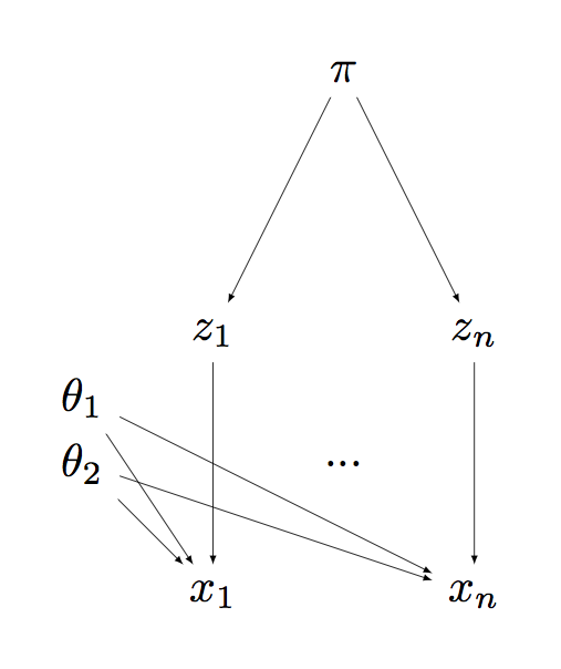
• In terms of density, this means our modelled density has the form: \begin{eqnarray} \phi = \pi \phi_{\theta_1} + (1 - \pi) \phi_{\theta_2}, \end{eqnarray} for $\pi \in [0, 1]$.
• Equivalently, we can write it in terms of auxiliary random variables $Z_i$, one of each associated to each measurement $X_i$: \begin{eqnarray} Z_i & \sim & \Cat(\pi) \\ X_i | Z_i, \theta_1, \theta_2 & \sim & \Norm(\theta_{Z_i}). \end{eqnarray}
• Each $Z_i$ can be interpreted as the sex of animal $i$.

Unfortunately, we did not record the male/female information when we collected the data!

• Expensive fix: Do the survey again, collecting the male/female information
• Cheaper fix: Let the model guess, for each data point, from which cluster (group, mixture component) it comes from.

Since the $Z_i$ are unknown, we need to model a new parameter $\pi$. Equivalently, two numbers $\pi_1, \pi_2$ with the constraint that they should be nonnegative and sum to one. We can interpret these parameters as the population frequency of each sex. We need to introduce a prior on these unknown quantities.

• Simplest choice: $\pi \sim \Uni(0,1)$. But this fails to model our prior belief that male and female frequencies should be close to $50:50$.
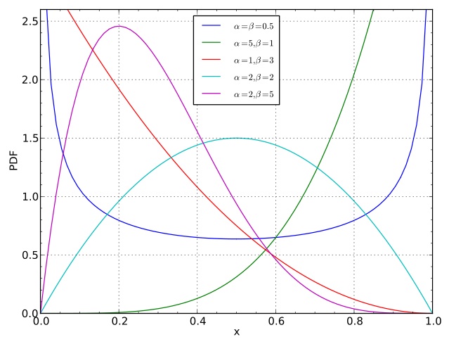
• To encourage this, pick a prior density proportional to: \begin{eqnarray} p(\pi_1, \pi_2) \propto \pi_1^{\alpha_1 - 1} \pi_2^{\alpha_2 - 1}, \end{eqnarray}
  where $\alpha_1 > 0, \alpha_2 > 0$ are fixed numbers (called hyper-parameters). The $-1$'s give us a simpler restrictions on the hyper-parameters required to ensure finite normalization of the above expression).
• The hyper-parameters are sometimes denoted $\alpha = \alpha_1$ and $\beta = \alpha_2$.
  • To encourage values of $\pi$ close to $1/2$, pick $\alpha = \beta = 2$.
  • To encourage this even more strongly, pick $\alpha = \beta = 20$. (and vice versa, one can take value close to zero to encourage realizations with one point mass larger than the other.)
  • To encourage a ratio $r$ different than $1/2$, make $\alpha$ and $\beta$ grow at different rates, with $\alpha/(\alpha+\beta) = r$. But in order to be able to build a bridge between Dirichlet distribution and Dirichlet processes, we will ask that $\alpha = \beta$

Dirichlet distribution: This generalizes to more than two mixture components easily. If there are $K$ components, the density of the Dirichlet distribution is proportional to: \begin{eqnarray} p(\pi_1, \dots, \pi_K) \propto \prod_{k=1}^{K} \pi_k^{\alpha_k - 1}, \end{eqnarray} Note that the normalization of the Dirichlet distribution is analytically tractable using Gamma functions $\Gamma(\cdot)$ (a generalization of $n!$). See the wikipedia entry for details.

Supplementary references

Robert, C. (2007) The Bayesian Choice. Most relevant to this lecture is chapter 10.