Instructor: Alexandre Bouchard-Côté
Editor: Sean Jewell

Review

We saw last time that a central goal in Bayesian model selection is to compute marginal likelihoods $m(x)$ and Bayes factors $B_{12}$. This is generally not as direct as computing posterior expectations, especially when both continuous and discrete distributions are involved. We talked about two methods last time: conjugate calculations, and model saturation, each with their own pros and cons. Today, we will cover more methods.

Parenthesis: project idea

Given the complexity of Bayesian model selection method when both continuous and discrete distributions are involved, it is generally a good idea to try to reduce the problem to a fully discrete case. This reduction can be completed through analytic marginalization. Why? Opportunity for new models.

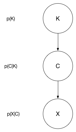
The following graphical model depicts the probabilistic relationship we are interested in modelling. $K$ denotes the number of clusters in the population, $C$ is a clustering viewed as a set of sets (e.g. $C = \{\{1,3\}, \{2\}, \{4,5,6\}\}$ for the points $\{1, 2, 3, 4, 5, 6\}$), and $X$ is the vector of observations. This project's goal is to build a Markov Chain over the clustering only!

Bayes factor, continued

Implementation of model saturation

We continue the example on the Poisson process models from last time. The goal is to select the model that best describes the data. The two models under consideration, Model 1 and Model 2, are given below.

\begin{align} & \mbox{Model 1} & & \mbox{Model 2} \\ \alpha &\sim \mathrm{exp}(0.1) & \beta_1, \beta_2 &\sim \mathrm{exp}(0.1) \\ x_1|\alpha &\sim \mathrm{Poi}(\alpha) & x_1|\beta_1 &\sim \mathrm{Poi}(\beta_1) \\ x_2|\alpha &\sim \mathrm{Poi}(\alpha) & x_2|\beta_2 &\sim \mathrm{Poi}(\beta_2) \end{align}

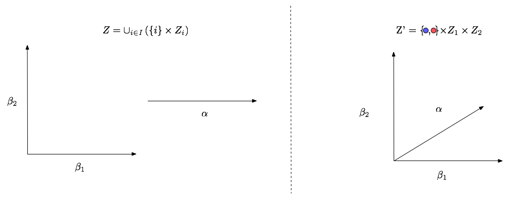
An issue with the standard formulation of the space $Z$ is that the union (depicted in the picture below) cannot be represented via a non-trivial graphical model (a graphical model with more than one node). To form a graphical model consider the construction $Z'$. This allows us to write:

\begin{align} \tilde{p}(\mu, z_1, z_2, x) &= p(\mu)p_1(z_1)p_2(z_2) \begin{cases} l_1(x|z_1) & \mu = 1 \\ l_2(x|z_2) & \mu = 2 \\ \end{cases} \end{align}

Importance sampling (IS)

We now consider the problem of evaluating the marginal likelihood of a single model (instead of a ratio). We start by looking at the more general issue of approximating integrals with importance sampling. Let $\pi(z)$ denote a density of interest, and $f(z)$, any (integrable) function. Our goal is to approximate $\int f(z) \pi(z) \ud z$. For example, we will take $f(z) = \ell(x | z)$, and $\pi(z)$ to be the prior here, since with this choice we have the evidence of $x$:

\begin{eqnarray} m(x) &= \int f(z) \pi(z) \ud z = \int \ell(x | z) \pi(z) \ud z. \end{eqnarray}

Suppose that $q(z)$ is a density whose support contains the support of $\pi(z)$. We assume that we can sample from $q$, or that we can sample from a Markov chain with stationary distribution $q$. $q$ is called the proposal distribution. Moreover, assume that we can compute $q(z)$ and $\pi(z)$ for any $z$ (including the normalization). We will relax this assumption later. Informally, the key idea behind importance sampling is: (1) to divide and multiply by $q(z)$: \begin{eqnarray} \int \;\; f(z) \pi(z) \ud z = \int \;\; f(z) \pi(z) \frac{q(z)}{q(z)} \ud z, \end{eqnarray}

(2) to re-interpret the above equation as an expectation with respect to $q$:

\begin{eqnarray} \int \;\; f(z) \pi(z) \frac{q(z)}{q(z)} \ud z &= \int f(z) w(z) q(z) \ud z \\ &= \E[w(\tilde Z) f(\tilde Z)], \end{eqnarray}

where $\tilde Z \sim q$ and $w(z) = p(z)/q(z)$, and (3) use the law of large numbers (LLN) to justify the following approximation:

\begin{eqnarray} \E[f(\tilde Z)w(\tilde Z)] \approx \frac{1}{N} \sum_{i = 1}^N f(\tilde Z^{(i)}) w(\tilde Z^{(i)}), \end{eqnarray}

where $\tilde Z^{(i)}$ could come from:

• iid samples from $q$ (justified using the standard LLN), or
• samples from a Markov chain with stationary density $q$ (Markov chain LLN).

---

Back to the marginal likelihood: a first choice would be $q(z) = p(z)$ (recall that we pick $f(z) = \ell(x|z)$ throughout this section). In this case, we get:

\begin{eqnarray} \frac{1}{N} \sum_{i = 1}^N \ell(x | z^{(i)}), \end{eqnarray}

however this does not work well in practice since the prior and posterior can be quite different. To improve on this, we will need a second version of importance sampling that does not require having access to the normalized density $q$.

---

Let us now relax the assumption that the normalization of both $q$ and $p$ are known. Let $\pi(z) = \gamma(z)/C_{\pi}$, where $\gamma(z)$ is easy to compute, but $C_{\pi}$ is hard. This will take care of the normalization of $q$ at the same time. Now use the same idea as above (1-3) to approximate:

\begin{eqnarray} C_{\pi} = \int \gamma(z) \ud z, \end{eqnarray}

obtaining the approximation:

\begin{eqnarray} C_{\pi} \approx \frac{1}{N} \sum_{i = 1}^N w'(\tilde Z^{(i)}), \end{eqnarray}

where $w'(z) = \gamma(z) / q(z)$.

Finally, invoking Slutsky justifies the approximation:

\begin{eqnarray} \frac{\frac{1}{N} \sum_{i = 1}^N f(\tilde Z^{(i)}) w'(\tilde Z^{(i)})}{\frac{1}{N} \sum_{i = 1}^N w'(\tilde Z^{(i)})} &= \frac{\sum_{i = 1}^N f(\tilde Z^{(i)}) w'(\tilde Z^{(i)})}{ \sum_{i = 1}^N w(\tilde Z^{(i)})} \\ &= \sum_{i = 1}^N f(\tilde Z^{(i)}) \bar w'(\tilde Z^{(i)}), \end{eqnarray}

where $\bar w$ denotes the normalized weights. Note also that in this final equation, $q(z)$ appears in both the numerator and denominator. Therefore, the approximation works with $w''(z) = \gamma(z) / u(z)$, where $q(z) = u(z) / C_q$.

---

Harmonic mean

Back to the marginal likelihood: Let us now take $u(z) = \ell(x|z) p(z)$, with $f(z) = \ell(x|z)$ to get:

\begin{eqnarray} \left( \frac{1}{N} \sum_{i=1}^N (\ell(x|z^{(i)}))^{-1} \right)^{-1} \end{eqnarray}

Unfortunately, the variance of this estimator is often infinite, resulting in very inefficient estimates.

Pro: easy to implement, does not require ratios.

Con: does not work reliably in practice. Avoid using this outside of a baseline for benchmarking other more sophisticated methods. See this blog entry by Radford Neal for an in depth example of the poor performance in estimating the marginal likelihood via the harmonic mean.

Bridge sampling

Exercise: assuming $\pi_i(z) = \gamma_i(z)/C_i$ for $i \in \{0, 1\}$, compute:

\begin{eqnarray} \frac{\E[\gamma_0(Z_1) h(Z_1)]}{\E[\gamma_1(Z_0) h(Z_0)]}, \end{eqnarray}

where $Z_i \sim \pi_i$, $h$ is an arbitrary function called a bridge function. A Monte Carlo estimator can be derived easily from the result of your calculation if $Z_i^{(j)}$ are distributed according to $\pi_i$ (or have $\pi_i$ as their stationary distribution in the MCMC case).

Note: this method is specialized to cases where the two models $\pi_0(z)$ and $\pi_1(z)$ are defined over the same space. One could in theory take $\pi_0$ to be the prior $p$, but in this case the method reduces to importance sampling.

Thermodynamic integration

As in bridge sampling, we target the ratio $B_{12}$, but we consider a continuum of intermediate distributions between $\pi_1$ and $\pi_2$. This opens the door to taking $\pi_0$ to be the prior $p$, with intermediate distributions $\pi_t = \gamma_t / C_t$, $t\in[0,1]$ given by $\gamma_t(z) = p(z) (\ell(x|z))^t$.

We start with the following standard identity, which holds under the assumption that we can swap a derivative and an integral (see for example Folland, Real Analysis):

\begin{align}\label{eq:thermo} \frac{\ud}{\ud t} \log C_t &= \frac{1}{C_t} \frac{\ud}{\ud t} C_t \\ &= \frac{1}{C_t} \frac{\ud}{\ud t} \int \gamma_t(z) \ud z \\ &= \frac{1}{C_t} \int \frac{\ud}{\ud t} \gamma_t(z) \ud z \\ &= \int \frac{1}{\gamma_t(z)} \frac{\ud}{\ud t} \gamma_t(z) \frac{\gamma_t(z)}{C_t} \ud z \\ &= \int \frac{\ud}{\ud t} \log \gamma_t(z) \pi_t(z) \ud z \\ &= \E_t\left[ \frac{\ud}{\ud t} \log \gamma_t(Z) \right], \end{align}

where $\E_t$ denotes expectation with respect to $Z \sim \pi_t$. We define $U_t(z) = \frac{\ud}{\ud t} \log \gamma_t(z)$.

Thermodynamic integration consists in integrating both sides of Equation (\ref{eq:thermo}) from 0 to 1, yielding:

\begin{eqnarray} \log C_1 - \log C_0 = \int_0^1 \E_t[U_t(Z)] \ud t. \end{eqnarray}

This can be approximated for example by numerical integration of the univariate integral, and Monte Carlo integration in the inner loop. See Lartillot, Nicolas, and Hervé Philippe for additional details.

---

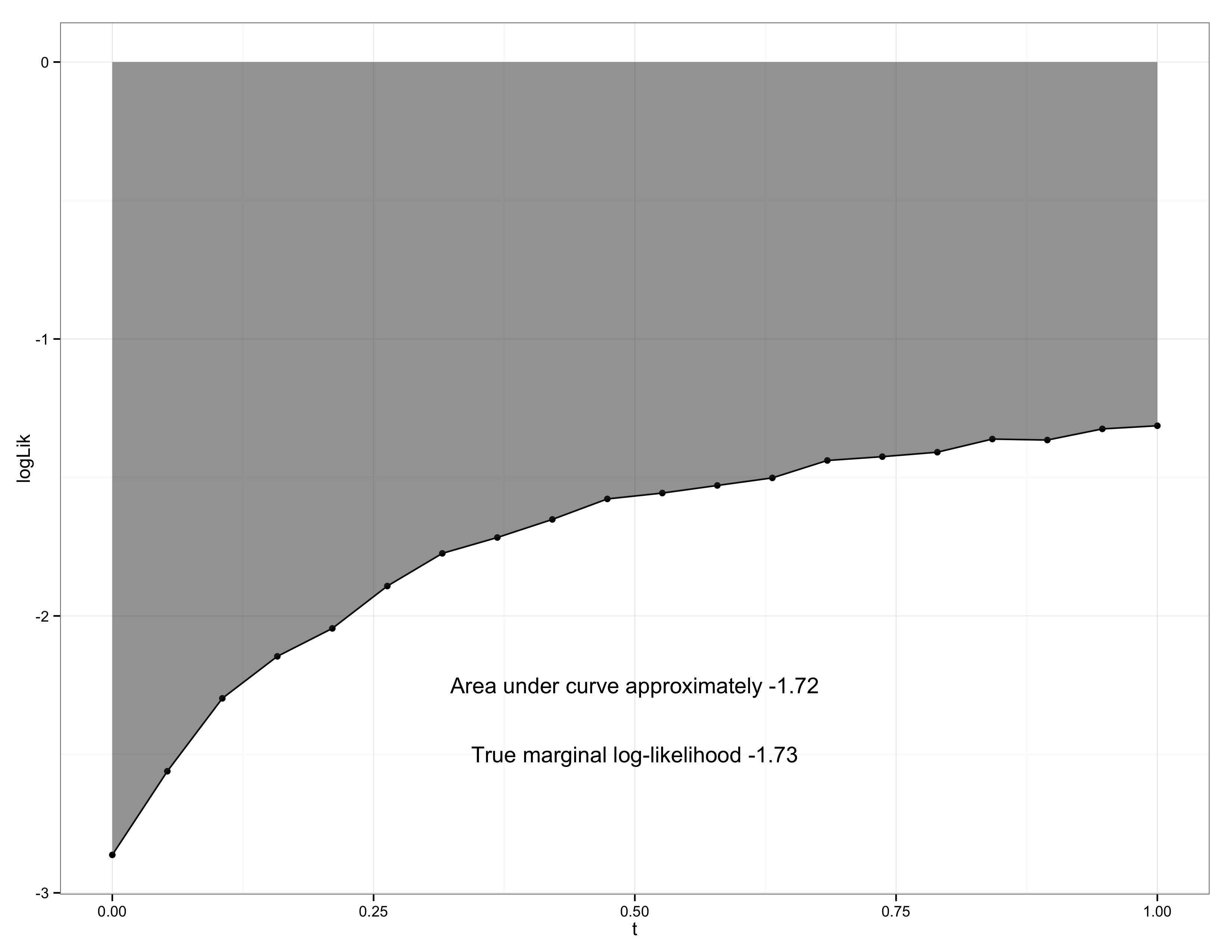
To showcase the performance gains of thermodynamic integration compared to the harmonic mean consider the example of Neal mentioned earlier. In this example the model is very simple:

\begin{align} \mu &\sim \mathrm{Normal}(0, s_0^2) \\ x &\sim \mathrm{Normal}(\mu, s_\1^2), \end{align}

so that the marginal distribution and posterior can be calculated exactly. Neal shows that the harmonic mean estimate performs very poorly. However, thermodynamic integration performs very well (see the figure below). In this figure the estimated values of $\E_t[U_t(Z)]$ are plotted for different $t$ and the integral $\int_0^1 \E_t[U_t(Z)] \ud t$ is performed via numerical methods (trapezoidal rule).

The corresponding code is downloadable as a Stan model and R file. See Carpenter, Bob, et al for a detailed description of user-defined probability distributions in Stan.

---

Pro: generally more accurate then the other methods.

Con: generally more computationally expensive.

Nested sampling

This method computes $C = m(x)$ from our usual Bayesian setup, $\pi(z|x) = p(z) \ell(x|z) / C$. Since the observation $x$ is fixed, let us abbrivate $\ell(x|z)$ by $\ell(z)$.

We will rewrite $C$ using the following standard formula: if $Y$ is a random variable with cdf $F(y)$, then:

\begin{eqnarray} \int_0^\infty (1 - F(y)) \ud y = \E[Y]. \end{eqnarray}

Example: write the expectation of a dice in two ways to get some intuition why this is true.

Let us apply this to the problem of computing $C$, which we can view as an expectation under the prior as follows:

\begin{eqnarray} C = \int p(z) \ell(z) \ud z = \E_p \ell(Z), \end{eqnarray}

where $Z \sim p$. Therefore, if we set:

\begin{eqnarray} G(\lambda) = \int_{\{z : \ell(z) > \lambda\}} \;\;\;p(z) \ud z, \end{eqnarray}

then:

\begin{eqnarray}\label{eq:nested1} C = \int_0^\infty\;\; G(\lambda) \ud \lambda. \end{eqnarray}

Equivalently:

\begin{eqnarray}\label{eq:nested2} C = \int_0^1\;\; G^{-1}(p) \ud p. \end{eqnarray}

(to see why this is equivalent, interpret each of the integrals in Equations (\ref{eq:nested1}) and (\ref{eq:nested2}) as an area under the curve.

Nested sampling is an approximation of the integral obtained via numerical integration on $[0, 1]$ paired with a Monte Carlo approximation scheme to approximate $G^{-1}(p)$.

Let us start by describing how the value of $G^{-1}(p)$ could be approximated for the largest $p$ in the numerical approximation:

1. Simulate $N = 10$ points $z_1, \dots, z_N$ according to the prior $p$.
2. Find the smallest likelihood value $\lambda_{\textrm{min}} = \min_i \ell(z_i)$. Let's say 0.007.
3. This suggests the approximation $G^{-1}(0.9) \approx 0.007$, since $G^{-1}(p) = \lambda$ if and only if $\P(\ell(Z) > \lambda) = p$ under the prior, $Z \sim p$.

Note that as $p$ gets smaller, we will generally want more and more closely spaced grid points.

So to get the second largest value of $G^{-1}(p)$, we will first add one more point. To make sure it is "useful", let us assume we can simulate one from the truncated prior,

\begin{eqnarray} p_\textrm{trunc}(z) \propto p(z) \1[z > \lambda_{\textrm{min}}]. \end{eqnarray}

This will give us an approximation for $G^{-1}\left( \left(\frac{N-1}{N} \right)^{2} \right)$.

Pro: can be more accurate then MCMC based methods.

Con: sampling from the truncated prior can be difficult.

Other methods for estimating Bayes factors

• Reversible jump MCMC.
• SMC samplers
• Chib's method

We might cover some of these later in the course.

Other model selection ideas

• Frequentist validation.
• Bayesian deviance.
• Classical approximations (BIC).

References

Neal, Radford. "The Harmonic Mean Of The Likelihood: Worst Monte Carlo Method Ever". Radford Neal's Blog 2008. Web. 19 Mar. 2015.

Carpenter, Bob, et al. "Stan: A Probabilistic Programming Language."

Lartillot, Nicolas, and Hervé Philippe. "Computing Bayes factors using thermodynamic integration." Systematic biology 55.2 (2006): 195-207.