Lecture 9: Particle MCMC and some theory
Instructor: Alexandre Bouchard-Côté
Editor: Json Hartford
Particle MCMC (PMCMC)
Motivation of pMCMC: estimating static parameters.
Example: change point detection.
Other motivations:
- Memory constrained inference.
- Basis for perfect simulation scheme.
Overview:
PMCMC methods are essentially MCMC algorithms in which SMC acts as a MH proposal. There is therefore an MCMC algorithm in the outer loop, indexed by $j$, and a SMC algorithm in the inner loop, with particle weights indexed by $w^{(j,k)}_n$.
In other words, we saw last week how to embed MCMC techniques inside SMC (i.e. adding via SMC samplers, some annealing and resample moves). Today is the other way around, using SMC techniques inside an MCMC sampler.
Simplest PMCMC algorithm: PMMH
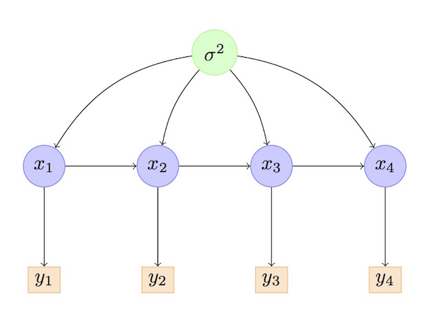
Suppose first we only care about getting a posterior over $\theta$ ($\sigma^2$ in the above example). Let $p(\theta)$ denote its prior density.
Difficulty: $Z_{\theta} = p(y | \theta)$, where $y$ is the data, is difficult to compute (recall that it would involve summing over all partitions $\rho$ of the $n$ datapoints).
On the other hand, for any fixed value of $\theta$, we can get an approximation of $Z_{\theta} = p(y | \theta)$ provided by running the SMC algorithm of the previous section and returning:
\begin{eqnarray} \label{eq:marg-smc} \hat Z^{(N)} = \prod_{t} \frac{1}{N} \sum_{i=1}^N w_t^i, \end{eqnarray}
where $t$ ranges over the SMC iteration where resampling was used, in addition to the last iteration, $N$ is the number of particles, and $w_t^i$ is $i$-th unnormalized weight at SMC iteration $t$.
Therefore, PMMH stores two quantities at each MCMC iteration $j$:
- A current value of the global variable $\theta^{(j)}$.
- An SMC estimate $Z^{(j)}$ corresponding to $\theta^{(j)}$, i.e. an approximation of the marginal density of the data given $\theta^{(j)}$.
At each MCMC iteration $j$, PMMH takes these steps:
- It proposes a new value for the global variable, $\theta'$, using a proposal $q(\theta'|\theta)$ (note the abuse of notation, $q$ is also used for the very different proposal used within the SMC inner loop).
- It computes an approximation $Z'$ to the marginal density of the data given $\theta'$ using Equation~(\ref{eq:marg-smc}).
- It forms the ratio: \begin{eqnarray} r = \frac{p(\theta')}{p(\theta)} \frac{Z'}{Z^{(j-1)}} \frac{q(\theta|\theta')}{q(\theta'|\theta)} \end{eqnarray}
- Sample a Bernoulli$(\min(1,r))$,
- If accepted, set $(\theta^{(j)}, Z^{(j)}) \gets (\theta', Z')$
- Else, set $(\theta^{(j)}, Z^{(j)}) \gets (\theta^{(j-1)}, Z^{(j-1)})$
Analysis:
For any fixed number of particles $N$, there will be an error in the approximation $Z^{(j)}$ of $Z_{\theta'}$. It follows that the MH ratio will be different than the idealized ratio, \begin{eqnarray} r^\star = \frac{p(\theta')}{p(\theta)} \frac{p(y|\theta')}{p(y|\theta)} \frac{q(\theta|\theta')}{q(\theta'|\theta)}, \end{eqnarray} and it is therefore not obvious a priori what is the asympotic behavior of PMMH if we let the number of MCMC iterations go to infinity for a fixed $N$.
It was therefore a surprise when Andrieu, Doucet and Holenstein, 2010 showed that even for fixed $N$ this converges to the right target, $p(\theta | y)$.
The basic idea is to introduce auxiliary variables modelling each step of the SMC inner loop, namely:
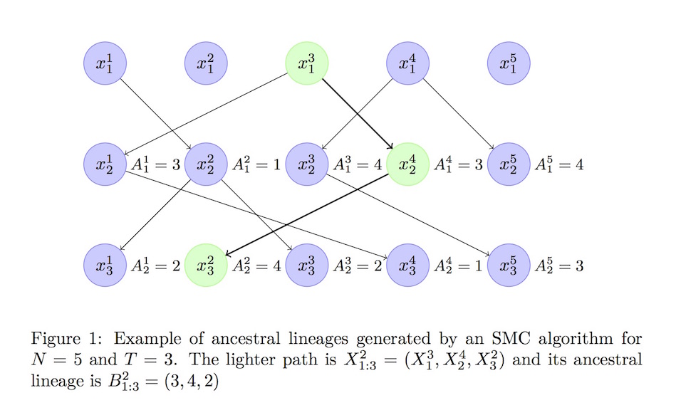
- $N(T-1)$ discrete variables $a = a_{1:T-1}^{1:N}$ on $\{1, \dots, N\}$ representing all the indices from the resampling steps (Resampling is not needed at the last iteration. why?).
- $NT$ variables representing the particles at all the SMC iterations.
- One extra random variable $\tau$ taking value from the $N^T$ particle resampling trajectories or ancestry $\{1, 2, \dots, N\} \times \dots \times \{1, 2, \dots, N\}$.
The auxiliary distribution we put on these random variables can be described with the following generative process:
- pick a value for the trajectory random variable $\tau$. This determines $T-1$ of the variables in $a$ at the same time.
- fill in the $T$ variables $v$ corresponding to the sampled trajectory according to the target (intractable) distribution $p(z|\theta)$.
- sample the rest of the variables according to the standard SMC algorithm (with the difference that the sampled trajectory is forced to be resampled at least once at each generation). Call $r$ this subset.
Appendix B1 of Andrieu, Doucet and Holenstein, 2010 shows that PMMH can be interpreted as a standard MH algorithm on that expanded space.
Some observations and background for understanding PMCMC:
- For pedagogy, assume the setup is based on a product space (see last lecture), and that the SMC proposal $q_{\textrm{SMC}}$ only depends on the previous state (e.g. think about an HMM), $q_{\textrm{SMC}}(x_n|x_{1:n-1}) = q_{\textrm{SMC}}(x_n|x_{n-1})$.
- Technically, we should have an index for the MCMC iteration $m$ as well, e.g. $(a_{1:T-1}^{1:N})^{(m)}$, but we drop it to avoid notation overdose.
- Let us ignore the static parameters $\theta$ to start with. They are easy to re-introduce.
- Review: Metropolis Hastings ratio.
- Background: genealogy.
This augmented construction also provides a second PMCMC algorithm called Particle Gibbs (PG). It corresponds to doing block sampling on the augmented space, with the sampling steps divided as follows:
- $\tau | \textrm{rest}$
- $r | \textrm{rest}$
- $\theta | \textrm{rest}$.
Again, see Andrieu, Doucet and Holenstein, 2010 for detail.
Supplementary references and notes
- Particle Markov chain Monte Carlo methods Andrieu, Doucet and Holenstein, Journal of the Royal Statistical Society: Series B, Vol. 72, Issue 3 (2010) , pp. 269-342.