Instructor: Alexandre Bouchard-Côté
Editor: Andres E. Sanchez-Ordonez

Based on: lecture 3 from last year.

Notation for a generic statistical problem

Consider the following generic statistical problem:

• we observe $x \in \Xscr$,
• we have a model of how this observation came to be in terms of some unknown quantities $z \in \Zscr$,
• and we want to make some decision (for example, reconstructing some of the unknown quantities, or forecasting future observations, etc).

More generally, we want to devise a decision-making strategy, which we formalize as an estimator: a function of the observation, $\delta(x)$.

We want this estimator to be as "good" as possible. Under a certain criterion of goodness, we will see that the Bayesian framework provides a principled and systematic way of specifying a "best" estimator.

Bayes estimators

Here is a very frequent misconception about the Bayesian framework that we will try to correct: "Bayesian methods consist of computing the posterior distribution and returning the point with the highest posterior density (1)." Other variants: "Bayesian methods consist of returning the posterior expectation of the parameters (2)."

While the posterior distribution is always involved in Bayesian methods, and that this posterior is sometimes used as in (1, 2) above, in other cases the Bayesian framework will prescribe other uses of the posterior.

How to use the posterior in general under the Bayesian framework is specified by the Bayes estimator.

In full generality, approaching a problem in a Bayesian way consists of:

1. specifying two quantities:
   • A model: which is simply a joint probability distribution $\P$ over the known and unknown quantities, modelled as random variables $X$ and $Z$ respectively.
   • A goal: specified by a set of actions $\Ascr$ (each action $a$ could be predictions, a decision, etc), together with a loss function $L(a, z)$, which specifies a cost incurred for picking action $a$ when the true state of the world is $z$. An important example, when $\Ascr$ coincides with the space of realization of $Z$, is $L(z', z) = (z - z')^2$, the squared loss.
2. selecting an estimator $\delta$ by minimizing the integrated risk, $\E[L(\delta(X), Z)]$.

Example where $\Ascr$ is different from the space of realization of $Z$?

Example from assignment 1.

Let $\Zscr$ denote the space of unknown parameters, $\Xscr$ denote the space of observations, and $\Ascr$ denote the set of possible actions. Furthermore, as described in assignment 1, let A denote the black background option, and B denote the white background option. Then, a model can be specified as follows:

• $X = (X_A, X_B) =$ (# clicks in A, # clicks in B)

• $Z = (Z_A, Z_B)$ where $Z_A, Z_B \in [0,1]$. We assume that $Z_A \sim Unif(0,1)$ and $Z_B \sim Unif(0,1)$

• $\Ascr = {A, B}$. That is, there are only two options, namely, A or B.

• $X_A | Z_A \sim Bin(N_A, Z_A)$ and $X_B | Z_B \sim Bin(N_B, Z_B)$ where $N_A = 51$ and $N_B = 47$

Finally, we choose a 0-1 loss such that $L(A,z) = \1[z_B > z_A]$ and $L(B, z) = 1 - L(A,z)$.

Discussion on the optimization in bullet point 2. Solving an optimization problem over a space of estimators seems quite abstract and hard to implement. Fortunately, it is possible to rewrite this optimization problem over the space of actions $\Ascr$. In other words, there is one general recipe for solving the above minimization problem:

Proposition: The estimator $\delta^*$, defined by the equation below, minimizes the integrated risk (in bullet point 2): \begin{eqnarray}\label{eq:bayes} \delta^*(X) = \argmin \{ \E[L(a, Z) | X] : a \in \Ascr \} \end{eqnarray}

This estimator $\delta^*$ is called a Bayes estimator.

This means that given a model and a goal, the Bayesian framework provides in principle a recipe for constructing an estimator.

Moreover, if the loss is strictly convex, the Bayes estimator is unique. See Robert 2007. In other words, under strictly convex losses, the Bayesian framework endows the space of estimators with a total order.

However, the computation required to implement this recipe may be considerable. This explains why computational statistics plays a large role in Bayesian statistics and in this course.

Example from assignment 1, continued.

In computing $\delta^*$ for the A-B testing example, note that

\begin{eqnarray} \E[L(\delta^*(X), Z)] = \int L(\delta^*(X(\omega), Z(\omega)) \P(\mathrm{d}\omega) \end{eqnarray}

so that

\begin{eqnarray} \delta^*(X) = \begin{cases} A &\mbox{if } \P(Z_A > Z_B|X) > \frac{1}{2} \\ \\ B & \mbox{otherwise } \end{cases} \end{eqnarray}

where

\begin{eqnarray} \P(Z_A > Z_B | X) = P(g(Z_A, Z_B) | X) = \int \int g(z_A, z_b) p(z_A, z_b| x) dz_A dz_B \end{eqnarray}

---

Note that other criteria certainly exist for selecting estimators, in particular frequentist criteria. Some of these criteria, such as admissibility, do not create a total order on the estimator (even under strictly convex losses), they only provide a partial order. Moreover, since the Bayes estimator can be shown to be non-suboptimal under this criterion as well (in other words, admissible).

Of course, these nice properties assume that the model is a true representation of the world (a well-specified model), a condition that is almost always false.

This provides a motivation for creating richer models that are more faithful to reality. In particular, models of adaptive complexity, that become progressively complex as more data become available. These models are called non-parametric (more formal definition below).

Bayesian estimation in parametric families

Many non-parametric models are built by composing a random number of parametric models (DP by themselves would be limited since it would predict duplicates in the observations, which we may not want). Parametric models are also very useful by themselves, for example for computational tractability reasons.

In the simplest cases, a parametric Bayesian model contains two ingredients:

1. A collection of densities over the observations $\Xscr$, indexed by the space of unknowns $\Zscr$. These densities are called likelihoods, $\Lscr = \{\ell(x | z) : z\in\Zscr\}$. The parametric assumption simply means that the collection is smoothly indexed by a subset of an Euclidean space, $\Zscr \subset \RR^d$ for some fixed integer $d$.
2. A prior density $p$ on $Z$._{Note: the random variables $X, Z$ are not necessarily continuous, so the densities $\ell$ and $p$ are defined with respect to some arbitrary (but fixed and known) reference measures. Since they do not play a central role in the theory, we will keep these reference measures anonymous, writing $\ud x, \ud z$ for integration with respect to these variables.}

---

Example: Consider a categorical likelihood model over two categories. This means that each individual observation $x_i$ is a point from a finite set of $k = 2$ objects. Let us denote the dataset by: $ x = (x_1, \dots, x_n), x_i \in \{\textrm{category 1, category 2}\}$. The parameter consists of two numbers $z = (z_1, z_2)$ that sum to one. This is a subset of $\RR^2$, therefore this is a parametric model. The value of the likelihood is given by:

\begin{eqnarray} \ell(x | z) = z_1^{n_1(x)} z_2^{n_2(x)}, \end{eqnarray}

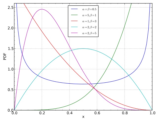
where $n_k(z)$ returns the number of times category $k$ was picked among the $n$ observations $x= (x_1, \dots, x_n)$ (since the likelihood only depends on the function $n = (n_1, n_2)$, we say that $n(\cdot) = (n_1(\cdot), n_2(\cdot))$ is a sufficient statistic). A suitable prior on $z$ is given by picking a Dirichlet distribution, with a density proportional to: \begin{eqnarray} p(z_1, z_2) \propto z_1^{\alpha_1 - 1} z_2^{\alpha_2 - 1}, \end{eqnarray}

where:

• $\alpha_1 > 0, \alpha_2 > 0$ are fixed numbers (called hyper-parameters).
• The $-1$'s give us a simpler restrictions on the hyper-parameters required to ensure finite normalization of the above expression.
• The hyper-parameters are sometimes denoted $\alpha = \alpha_1$ and $\beta = \alpha_2$.
  • To encourage values of $z$ close to $1/2$, pick $\alpha = \beta = 2$.
  • To encourage this even more strongly, pick $\alpha = \beta = 20$. (and vice versa, one can take value close to zero to encourage realizations with one point mass larger than the other.)
  • To encourage a ratio $r$ different that $1/2$, make $\alpha$ and $\beta$ grow at different rates, with $\alpha/(\alpha+\beta) = r$.
• A shortcut often used when there are two categories ($k = 2$) is to say that $z_1$ is Beta distributed, $z_1 \sim \textrm{Beta}(\alpha, \beta)$, and to set $z_2 = 1 - z_1$, which is completely equivalent to $(z_1, z_2) \sim \textrm{Dir}(\alpha, \beta)$.
• An even more special case is when $\alpha = \beta = 1$, in which case $z_1$ and $z_2$ are uniform (but not independent, $z_2 = 1 - z_1$).

---

In order to evaluate our objective function, Equation~(\ref{eq:bayes}), we need to compute posterior expectations of the form $\E[\phi(Z)|X]$, where $\phi(z) = L(a,z)$ for some $a$ that we consider fixed for now.

Let us denote the posterior density by $p(z|x)$. We need to compute:

\begin{eqnarray}\label{eq:posterior} \int \phi(z) p(z|x) \ud z. \end{eqnarray}

By Bayes rule, this posterior density is proportional to the joint density (up to null sets), in other words, proportional to a prior times a likelihood (chain rule):

\begin{eqnarray} p(z|x) \propto p(z) \ell(x|z), \end{eqnarray}

with the following normalization for the right-hand side:

\begin{eqnarray}\label{eq:marginal} m(x) = \int p(z) \ell(x|z) \ud z. \end{eqnarray}

This normalization, denoted by $m(x)$, is called the marginal likelihood or evidence. If the observations $x$ are discrete, this corresponds to the probability of the observed dataset under the model. For this reason, the evidence plays an important role in Bayesian model selection.

The integrals in Equations~(\ref{eq:posterior}, \ref{eq:marginal}) constitute one of the main challenge in Bayesian inference. We will discuss two approaches to solve these integrals in this course.

• Approximating the integral via approximation methods (MCMC, SMC, variational, etc; more on that later).
• Picking the prior and likelihood so that analytic computations are possible (described in the next section).

Conjugacy in parametric families

Let us say that we are given a fixed likelihood model $\Lscr$. Our strategy to ensure tractable expressions in Equations~(\ref{eq:posterior}, \ref{eq:marginal}) consists in constructing a family of distributions over $z$, $\Cscr = \{p_h\}$ (where $h \in \mathbb{R}^d$ is an index called a hyper-parameter), such that:

1. The prior density is in this family: $p = p_{h_0} \in \Cscr$
2. More generally, given any observed dataset $x$, the posterior density should be a member of the conjugate family: $p(z|x) = p_{h'}(z) \in \Cscr$ for some updated hyper-parameters $h'$.

Finding a collection that satisfies these two conditions is easy. For example, if $\Lscr$ is an exponential family with $k$-dimensional parameters, it is always possible to find a conjugate family with $(k+1)$-dimensional parameters (see this hand-out). Note also that trivially, the class of all distributions is conjugate to any likelihood model.

But in order for the conjugate approach to be computationally feasible, we should also ensure that:

• Each member $p_h$ of the family should be tractable, in particular we should have an efficient algorithm for computing the normalization constant of arbitrary members.
• We should also have an efficient algorithm for finding updated parameters $h'$, as a function of the observed data $x$ and prior hyper-parameters $h_0$, $h' = u(x, h_0)$.

---

Example (continued): the Dirichlet distributions with hyperparameters $h = \alpha$ are conjugate to the multinomial likelihood. Moreover, the Dirichlet-multinomial model has the two nice computational tractability properties listed above.

Recall that for any hyper-parameter vector $h = \alpha$, a distribution on the simplex proportional to $z_1^{\alpha_1-1} z_2^{\alpha_2-1}$ has a known normalization $N(\alpha)$, namely

\begin{eqnarray}\label{eq:dir-norm} p_\alpha(z) & = & \frac{z_1^{\alpha_1-1} z_2^{\alpha_2-1} }{N(\alpha)} \\ N(\alpha) & = & \frac{\Gamma(\alpha_1) \Gamma(\alpha_2)}{\Gamma(\alpha_1 + \alpha_2)}. \end{eqnarray}

Now let us look at the form of the posterior (up to normalization):

\begin{eqnarray}\label{eq:dir-prop} p(z | x) & \propto & p_\alpha(z) \ell(x | z) \\ & \propto & z_1^{n_1(x) + \alpha_1 - 1} z_2^{n_2(x) + \alpha_2 - 1}. \end{eqnarray}

To conclude, we use the simple but extremely useful fact that if two densities are proportional (in this case, Equation~(\ref{eq:dir-norm}) and (\ref{eq:dir-prop})), then they are equal (up to null sets). By Equation~(\ref{eq:dir-norm}), we can therefore conclude that the hyper-parameters update is given by $u(x, \alpha) = \alpha + n(x)$.

Connect with first question of assignment 1.

For the A-B testing example under the formulation above, we have the following posterior:

\begin{eqnarray} p(z|x) = \frac{\Gamma(\alpha_1 + \alpha_2 + n_1(x) + n_2(x))}{\Gamma(\alpha_1 + n_1(x))\Gamma(\alpha_2 + n_2(x))} \end{eqnarray}

where $n = n_1(x) + n_2(x)$. Then, it follows that

\begin{eqnarray}\label{eq:AB-testing-int-risk} \P(Z_A < Z_B | X)=\int \int p(z_A, z_B | X) \1[z_A < z_B] dz_A dz_B \end{eqnarray}

We can further decompose the joint posterior $p(z_A, z_B | X) = p(z_A | X)p(z_B | X)$ and after appropriate substitution find Equation \ref{eq:AB-testing-int-risk} to be

\begin{eqnarray} \int \int \frac{1}{N(\alpha_A')} \frac{1}{N(\alpha_B')} z_A^{\alpha_A' -1} (1-z_A)^{\beta_A' - 1} z_B^{\alpha_B' -1} (1-z_B)^{\beta_B' - 1} dz_A dz_B \end{eqnarray}

where $N(\alpha_A')$ is the normalising constant for a Dirichlet distribution, $n_1(\cdot)$ denotes a click, $n_2(\cdot)$ denotes no click, $\alpha_A' = 1 + n_1(X_A), \beta_A' = 1 + n_2(X_A),$ and similarly for $\alpha_B'$ and $\beta_B'$.

Although the A-B testing problem is now fully specified in analytical form, solving Equation~\ref{eq:AB-testing-int-risk} directly is not practical. Therefore, we solve the problem via a Monte Carlo approximation from the posterior.

Let $z^{(i)} = (z_A^{(i)}, z_B^{(i)})$ denote the imputed latent states for $i = 1, 2, \dots, N$ with corresponding weights $w^{(i)} \in [0,1]$. For MCMC, the weights are simply $w^{(i)} = 1/N$ such that $\sum_i w^{(i)} = 1$(weights in SMC are covered in later lectures). Then,

\begin{eqnarray} \E[g(Z)|X] = \sum_i^N w^{(i)} g(z^{(i)}) \end{eqnarray} where

\begin{eqnarray} \sum_i^N W^{(i)} g(Z^{(i)}) \rightarrow \E[g(Z)|X]. \end{eqnarray}

Note that we used upper case $W$ and $Z$ since this convergence is based on the random quantities.

---

Another important example of a conjugate family is the normal-inverse-gamma distribution. Please read this article.

One final note that we will use later: tractable conjugacy also gives us a way of computing the evidence $m(x)$. This is done by rearranging Bayes rule:

\begin{eqnarray} m(x) & = & \frac{p_{h}(z) \ell(x | z)}{p(z | x)} \\ & = & \frac{p_{h}(z) \ell(x | z)}{p_{u(x, h)}(z)}. \end{eqnarray}

Since this is true for all $z$, we can pick an arbitrary $z_0$, and evaluate each component of the right-hand side by assumption.

Supplementary references and notes

Robert, C. (2007) The Bayesian Choice. An excellent textbook, especially for the theoretically foundations of Bayesian statistics. Also covers many practical topics. Most relevant to this course are chapters 2, 3.1-3.3, 4.1-4.2.

van der Vaart, A.W. (1998) Asymptotic Statistics. Chapter 10 contains a formal treatment of the asymptotic properties of parametric Bayesian procedures. Note that a different treatment is needed for non-parametric Bayesian procedures.