Lecture 11: From model selection to Bayesian non-parametrics
Instructor: Alexandre Bouchard-Côté
Editor: TBA
Prerequisites
- Two simulation concepts in Bayesian statistics: recall that a Bayesian model specifies a joint distribution on the known $Y$ and unknown $X$.
- Posterior simulation: $X \mid Y$
- Forward simulation: $(X, Y)$.
- Today, we will focus on mixture models, which is an important source of Bayesian non-parametric models (but not the only one!)
Model selection vs. Bayesian non-parametric models
- We will contrast forward simulation in the two models.
- Let $P_n$ denote the number of parameters used to generate $n$ datapoints ($\propto$ the number of distinct clusters)
- Let $P = \lim_{n\to \infty} P_n$
- Note: $P_n$ are $P$ are random!
- Distinction:
- Bayesian parametric model: $\P(P = \infty) = 0$
- Bayesian non-parametric model (BNP): $\P(P = \infty) > 0$.
- Examples of applications where model selection/BNP is preferred:
- Model selection: clustering, cases where the parametric component is a good approximation.
- BNP: density estimation, especially when the parametric model is not trusted. Phenomena with fat tails, e.g. frequency of words (do you think assuming the number of existing words is finite is a good idea?)
However, note that for posterior simulation, the number of parameters is bounded by the number of datapoints, therefore similar MCMC techniques can be used in both cases (in particular, RJMCMC probably have been underused in BNP posterior inference).
Viewing clustering priors as random probability distributions
- Let us say we are given a set $A \subset \RR \times (0, \infty)$
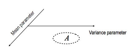
- The space $\RR \times (0, \infty)$ comes from the fact that we want $\theta$ to have two components, a mean and a variance, where the latter has to be positive
- Let us call this space $\Omega = \RR \times (0, \infty)$
- We can define the following probability mesure
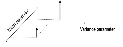 \begin{eqnarray}
G(A) = \sum_{k=1}^{K} \pi_k \1(\theta_k \in A),
\end{eqnarray}
where the notation $\1(\textrm{some logical statement})$ denotes the indicator variable on the event that the boolean logical statement is true. In other words, $\1$ is a random variable that is equal to one if the input outcome satisfies the statement, and zero otherwise.
\begin{eqnarray}
G(A) = \sum_{k=1}^{K} \pi_k \1(\theta_k \in A),
\end{eqnarray}
where the notation $\1(\textrm{some logical statement})$ denotes the indicator variable on the event that the boolean logical statement is true. In other words, $\1$ is a random variable that is equal to one if the input outcome satisfies the statement, and zero otherwise.
Random measure: Since the location of the atoms and their probabilities are random, we can say that $G$ is a random measure. The Dirichlet distribution, together with the prior $p(\theta)$, define the distribution of these random discrete distributions.
Another view of a random measure: a collection of real random variables indexed by sets in a sigma-algebra: $G_{A} = G(A)$, $A \in \sa$.
Limitation of our setup so far: we have to specify the number of components/atoms $K$. The Dirichlet process is also a distribution on atomic distributions, but where the number of atoms can be countably infinite.
Dirichlet processes and other random probability distributions
Definition: A Dirichlet process (DP), $G_A(\omega) \in [0, 1]$, $A \in \sa$, is specified by:
- A base measure $G_0$ (this corresponds to the density $p(\theta)$ in the previous example).
- A concentration parameter $\alpha_0$ (this plays the same role as $\alpha + \beta$ in the simpler Dirichlet distribution).
To do forward simulation of a DP, do the following: 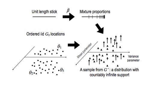
- Start with a current stick length of one: $s = 1$
- Initialize an empty list $r = ()$, which will contain atom-probability pairs.
- Repeat, for $k = 1, 2, \dots$
- Generate a new independent beta random variable: $\beta \sim \Beta(1, \alpha_0)$.
- Create a new stick length: $\pi_k = s \times \beta$.
- Compute the remaining stick length: $s \gets s \times (1 - \beta)$
- Sample a new independent atom from the base distribution: $\theta_k \sim G_0$.
- Add the new atom and its probability to the result: $r \gets r \circ (\theta_k, \pi_k)$
Finally, return: \begin{eqnarray} G(A) = \sum_{k=1}^{\infty} \pi_k \1(\theta_k \in A), \end{eqnarray}
This is the Stick Breaking representation, and is not quite an algorithm as written above (it never terminates), but this can be fixed by lazy computing.
Other examples:
- Pitman-Yor. Make the parameters of the beta depend on the level (at level $i$, use $(1-d, \alpha + id)$, where $d$ is a tuning parameter $d \in [0, 1)$.
- Normalized random measures (in particular, normalized generalized gamma, which includes Normalized inverse gaussian, DP, normalized stable).
- Most general category, Exchangeable Partition Probability Functions (EPPF) not believed to be tractable.
Key motivation for these extensions: DPs can give us $P_n \sim \log(n)$. PY gives us $P_n \sim n^d$. PY also yields a power law distribution on the number of customers per table (i.e. the number $m$ of customers is proportional to $m^{-(1+d)}$ (truncated to avoid the asymptote at zero).