Lecture 13: BNP, continued
Instructor: Alexandre Bouchard-Côté
Editor: TBA
Hierarchical DP (HDP)
Motivation: N-gram Language models
N-gram language models are a type of distributions over sequences of words (where a word is viewed as an abstract symbol $w$ from a finite set $W$, called the alphabet). Sequences of words are often called strings. We denote the set of all possible strings by $W^\star$. For example, if $W = \{$a, b$\}$, then $W^\star=\{\epsilon,~$a, b, aa, ab, ba, bb,$\dots\}$, where $\epsilon$ is the empty string. With this notation, N-gram language models can be described as the probability distributions $\lmodel_k$ over $W^\star$, which can be written as:
\begin{eqnarray} \lmodel_k(\underbrace{w_0,\ldots,w_k}_{w\in W^*})= \prod^{k}_{i=1}\lmodel(\underbrace{w_i}_{\textrm{given word}}|\underbrace{w_{i-n}\ldots w_{i-1}}_{\textrm{prefix of length } n}) \end{eqnarray}
The integer $n$ is fixed, and is called the order of the language model. Here we assume $n=1$, i.e. only the previous word is conditioned upon—this is called a unigram model. The right hand side of the conditioning is called the context.
Language models are used to find which sentence is more likely. To understand why this is useful, here we present a very simplified version of speech recognition model. The task in speech recognition is to estimate a sequence of words corresponding to a sequence of sounds $s$.
In the HMM over words, we have $w_{t+1}|w_{t} \sim \lmodel_1$, while the sound unit given a word, $s_t|w_t$ is modeled by another HMM, this time over smaller signal segments. In practice, the boundary between words are not known (which complicates the model), but the general idea of how language models are used is the same: to disambiguate between similar-sounding words.
For example, the words 'their' and 'there' cannot be told apart from their pronunciation, but they can usually be differentiated by the context in which they are used. Note also that language models can be trained on raw text (which is cheap and available in large quantity online, e.g. from Wikipedia), while training $s_t|w_t$ requires annotated speech data (expensive).
Estimation of language models:
The direct, naive approach to build an n-gram model $\lmodel_1$ is to parameterize each of the $|W|$ multinomial distributions $\lmodel_1(w_i|w_{i-1})$ by a separate vector of parameters, and to estimate these parameters independently using maximum likelihood.
The problem is that this approach results in zero probability for pairs which we have not seen before, even when each word in the pair has been seen (in different contexts). For example, the sequence 'I think' may be given zero probability even though 'they think' and 'I believe' have been observed. This can have dramatic effect in, say, a speech recognition system: a long sentence would be given probability zero even when a single pair has not been seen. Note that in contrast, a context-free model (i.e. an n-gram language model with $n=0$) would give a positive probability to 'I think' given this training data because each word has been observed.
Since the training data is more fragmented to higher order language models, there should be some mechanisms to back off to simpler models. We will accomplish this using a model called the hierarchical Dirichlet process (HDP) (Teh et al., 2004). For pedagogical reasons, before introducing the HDP, we will start by showing how a simple Dirichlet process model as introduced in the previous set of notes could be used to back off to a fixed model (e.g. uniform distribution over words). Next, we will show how the HDP can provide more intelligent back-off distributions, namely lower order n-gram models.
Language model using DPs:
To address the aforementioned problem, we introduce the following model, a Dirichlet process with base measure equal to the uniform distribution over $W$: \begin{eqnarray} \pi^u &\sim& \gem(\alpha_0) \ \textrm{(stick breaking dist.)}\\ \theta^{u}_{c} &\sim& G_0 \ \textrm{where } G_0 = \unif(W)\\ x^{u}_{n}|\pi^u &\sim& \mult(\pi^u)\\ y^{u}_{n}|x^{u}_{n},\theta^{u} &\sim& \delta_{(\theta^{u}(x^{u}_{n}))} \end{eqnarray} Here $y^{u}_{i}$ is a word following prefix $u$ (from now on, we use the superscript to annotate the prefix/context under which the next word has to be predicted), and $\delta_{(\theta^{u}(x^{u}_{n}))}$ is the Dirac delta function.
In the directed graphical model notation, this looks like the following:
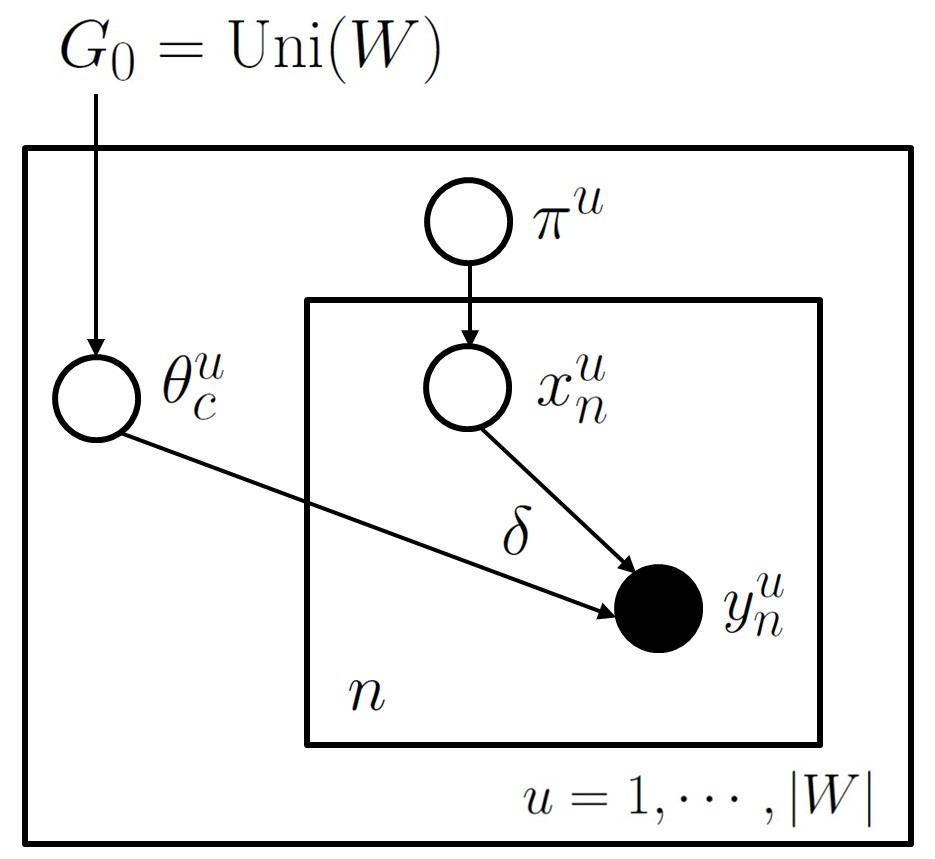
A more compact way to write this is: \begin{eqnarray} G^{u} &\sim& \dirp(\alpha_0, \unif(W))\\ y^{u}_{n}|G^{u} &\sim& G^u. \end{eqnarray}
Note that, in contrast to the previous mixture modeling/clustering example, the likelihood model here is a simple, deterministic function of the dish for the table: a Dirac delta on that dish. Concretely, a dish is a word type, and customers simply have this word associated with them deterministically. This implies that, given a table assignment, the dishes at each table are observed, which simplifies probabilistic inference.
Note that this model never assigns a zero probability to words in $W$ (even when the word was not observed in the context) since the probability of a new word (i.e. creating a new table in CRP) is positive. Now suppose we have the following observations and table assignments for one of the contexts $u$:
\begin{eqnarray} x^{u}_{1} \ldots x^{u}_{n} &\longleftarrow& \textrm{table assignments} \\ w^{u}_{1} \ldots w^{u}_{n} &\longleftarrow& \textrm{words} \end{eqnarray}
then it can be shown (easy exercise) that generating a new word is done using the following probabilities:
\begin{eqnarray} \underbrace{w^{u}_{n+1}}_{\textrm{new customer}}|x^{u}_{1},\ldots,x^{u}_{n} &\sim& \textrm{1. create new table; dish sampled from } G_0\textrm{ with prob.} \frac{\alpha_0}{\alpha_0+n} \textrm{, OR,} \\ && \textrm{2. use a dish } w \textrm{ from existing tables with prob.} \frac{n^{u}_{w}}{\alpha_0+n} \end{eqnarray} in which $n^{u}_{w}$ is the number of times $w$ was observed in all the training data $w^{u}_{1} \ldots w^{u}_{n}$.
Note that in this setting, to do prediction we only need to know, for each context, the number of times each word appeared in the text. Consequently, we can marginalize the table assignments and there is no MCMC sampling required in this special case (this will not be true in the following models).
HDP models
A problem with the approach of the previous section is that the back-off model, the uniform distribution, is not very good. A better option would be to back off to a context-free distribution over words. One way to achieve this is to use the MLE over words in the corpus instead of the uniform distribution as the base measure. This approach is called the empirical Bayes method. Here we explore an alternative called the hierarchical Bayesian model.
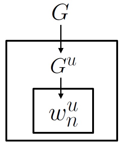
The basic idea behind HDPs is to let the base measure be itself a Dirichlet process: \begin{eqnarray} G &\sim& \dirp(\alpha_0, \unif(W))\\ G^u|G &\simiid& \dirp(\alpha^{u}_{0}, G)\\ w^{u}_{n}|G^{u} &\sim& G^{u} \end{eqnarray}
In the directed graphical model notation, this looks like (recall that boxes, called plates, mean repetition of the variables inside the box) the following:
To make this model clearer, we will provide two equivalent ways of generating samples from it: as in the standard DP, both stick breaking and CRP constructions are possible.
Let us start with the stick breaking way. We will describe the generative process by referring to the following figure:
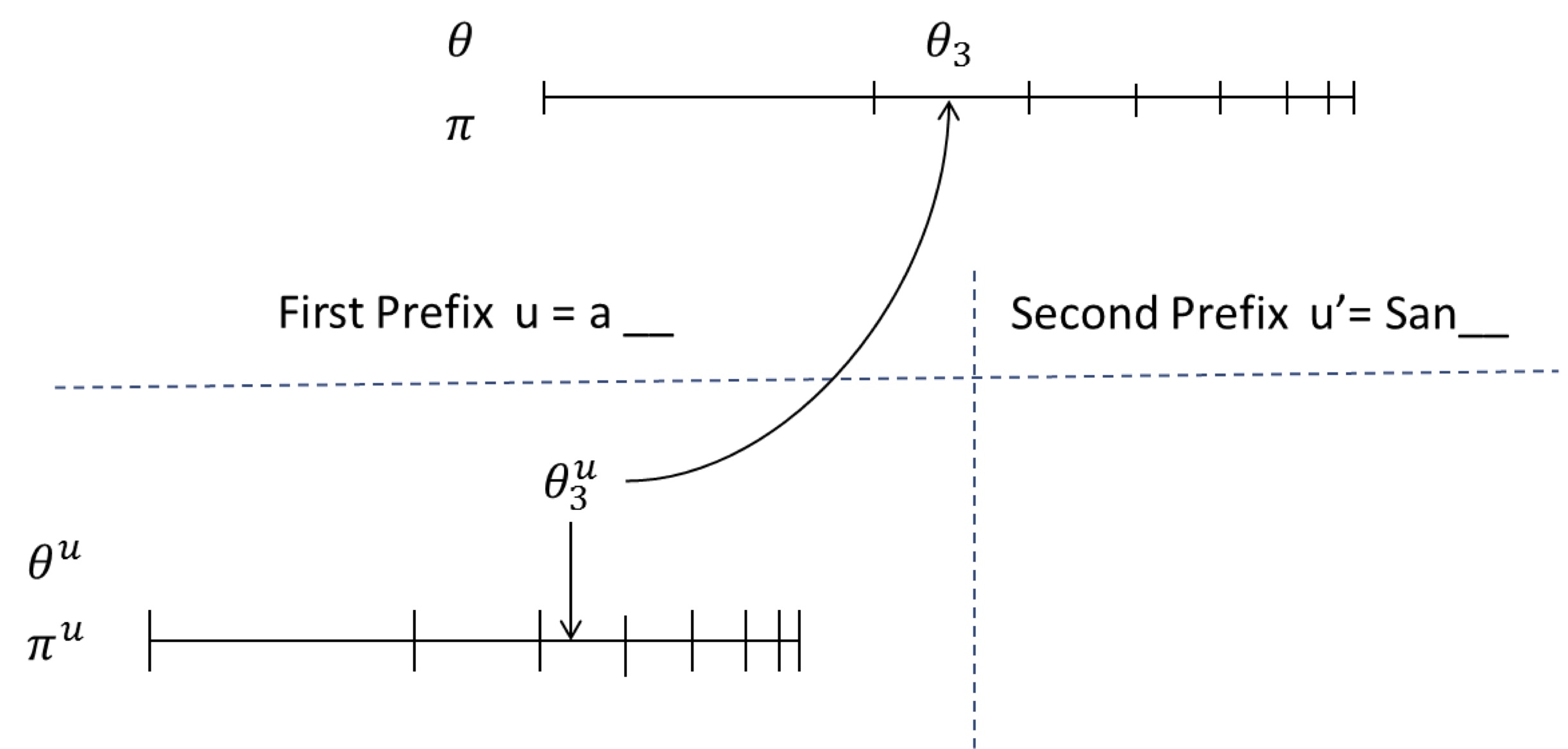
There is one set of sticks for each prefix (one of them is shown below the horizontal dashed line), and one global set of stick (above the horizontal dashed line) corresponding to the context-free model.
To sample from the first prefix in the figure above:
- Throw a dart on the prefix-specific stick $\pi^u$
- If it ends up in segment $c$ (e.g. $c=3$ here), sample $c$ beta random variables to construct the first few sticks
- Extract $c$ samples from $G$, return the third one. $G$ can be sampled from using the following steps (the usual DP):
- Throw a dart on $\pi$,
- If it end up in segment $c'$ (e.g. $c'=2$ here), sample $c'$ beta random variables to construct the first few sticks
- Generate $\theta_1, \dots, \theta_{c'}$ from $\unif(W)$. Here $\theta_{c'}$ is the first realization of $G$. Repeat the process to generate $c=3$ realizations from $G$. Return $\theta_3$.
When the next sample is needed, only generate new sticks and base measure samples if the dart falls outside the region that was generated so far. This means that samples from $G_0$ are needed only when both the dart on the context specific and global sticks fall outside the sticks already generated.
Another way to view this process is the Chinese Restaurant Franchise. In the Chinese restaurant franchise, the metaphor of the Chinese restaurant process is extended to allow multiple restaurants to share a set of dishes.
We will refer to the following figure:
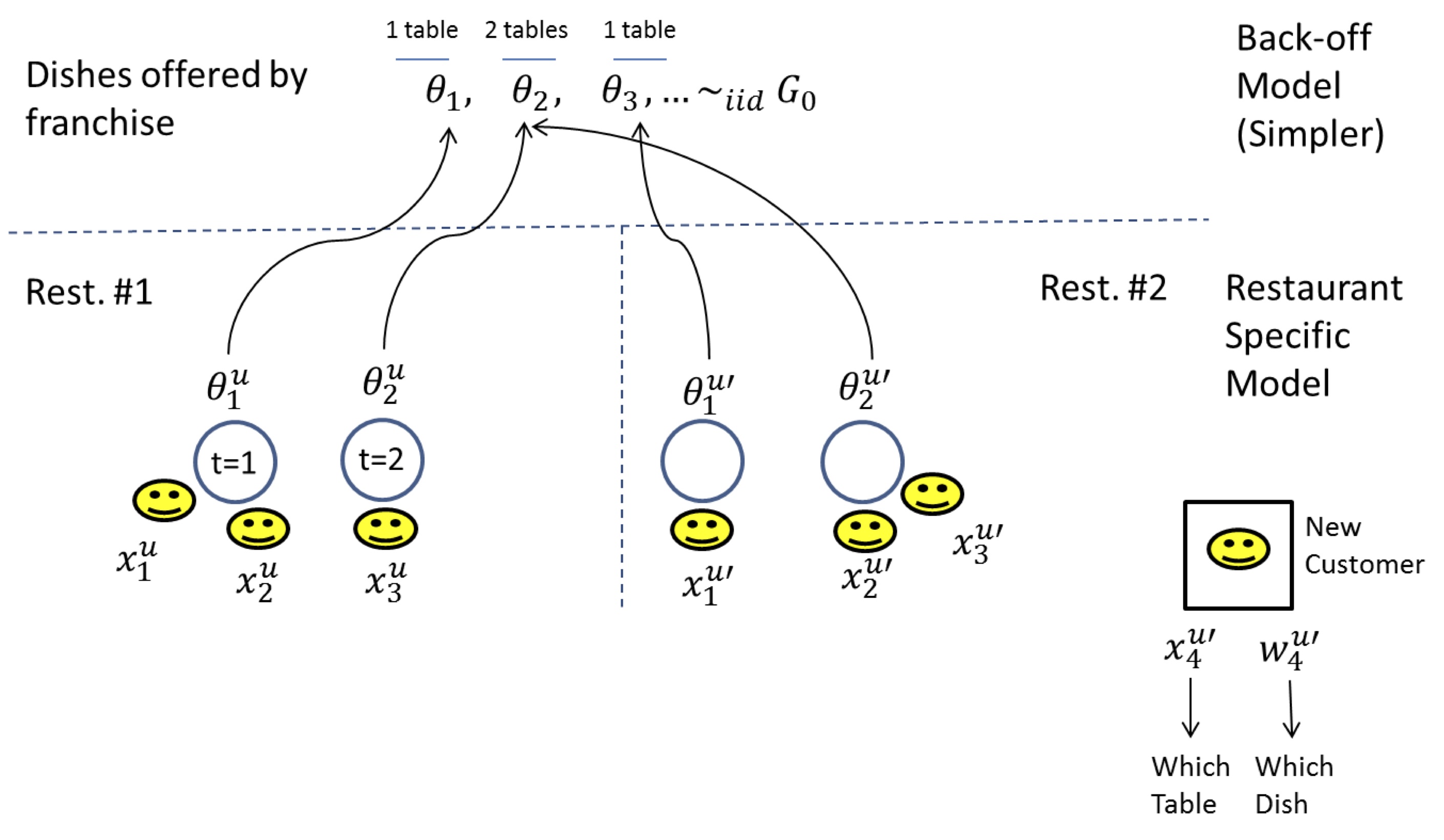
Here each context (prefix) corresponds to a restaurant. The same dish can be served across many restaurants (hence the franchise terminology).
For a new customer entering say in the second restaurant (i.e. $x^{u'}_{4},w^{u'}_{4}|x^{u'}_{1:3},w^{u'}_{1:3},x^{u}_{1:3},w^{u}_{1:3}$) the sampling process can be summarized by the following decision tree:
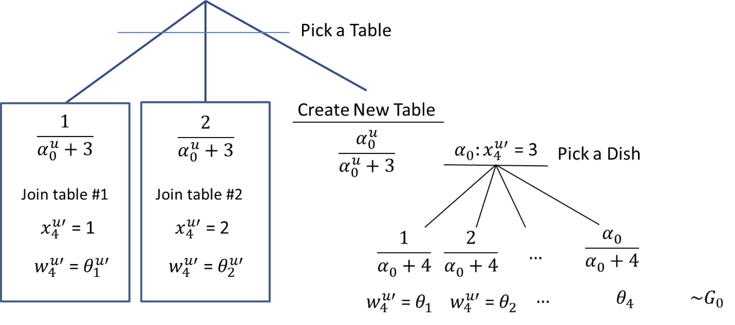
In other words, the customer first picks if he will join an existing table in the current restaurant (with probability proportional to the number of people at that table), or create a new table (with probability equal to $\alpha^{u}_0/(n_{\textrm{cust. in rest.}}+\alpha^{u}_0)$, where $n_{\textrm{cust. in rest.}}$ is the number of customers in the current restaurant). In the former case, the dish is the same as the one served at the picked table, in the latter case, another dish needs to be sampled. It has the same structure, but this time existing dishes are sampled with probability proportional to the number of tables that picked that dish, across all restaurants. A new dish can also be sampled with probability equal to $\alpha_0/(n_{\textrm{tables}}+\alpha_0)$, where $n_{\textrm{tables}}$ is the number of tables across all restaurants.
Deeper and infinite hierarchies
Why stop at two level? In many practical situations, models can perform better by considering deeper hierachies. This is true in particular for language modelling, where prefixes of length 0, 1, 2, 3, 4 and more are common.
As the hierarchies go deeper, you will more and more see cases where a $G^u$ has a single child $G^{u'}$. When we have this twice in a row, $G^u \to G^{u'} \to G^{u''}$ can we simplify to $G^u \to G^{u''}?
The answer is yes, if the model is a certain type of Pitman-Yor process:
If $G^{u''} | G^{u'} \sim \textrm{PY}(0, d_1)$ and $G^{u'} | G^{u} \sim \textrm{PY}(0, d_2)$, then $G^{u''} | G^{u} \sim \textrm{PY}(0, d_1 d_2)$.
Note that each conditional can $G^{u''} | G^{u'}$ and $G^{u'} | G^{u}$ can be viewed as a so called coagulation operator, where clusters are merged by having the table pick the same dish in the franchise.
HDP + mixture = HDP-HMM
- Consider a Bayesian HMM on $K$ states
- Let us place a Dirichlet prior on each row $\pi^u$ of the transition matrix.
- The rest of the HMM is the same as before (assume a known likelihood $\ell(\cdot\mid \theta)$ and prior $G_0$ for the state specific priors $\theta_1, \dots, \theta_K$.
- It is also reasonable to consider a hierarchical model for the $\pi^u$, say centered on a shared $\pi$, itself Dirichlet distributed.
- An HDP-HMM simply replaces the Dirichlet priors by GEM priors.
Some options for inference:
- Gibbs sampling on the CRF representation.
- Methods on the stick breaking representation: beam sampling
- Particle MCMC
Practical considerations:
- The HDP-HMM does not have any special consideration for self-transition. It is often useful to inflate these in practice: sticky HDP-HMM
- A continuous time version of this process that came out from this course: the Gamma-Exponential Process
- Note that the HPD prior assigns mass to processes that are non-reversible. Also, the global variable $\pi$ is not the stationary distribution. Alternatives to HPD-HMM: edge reinforced random walk, SHGP
More pointers
- nested Dirichlet processes
- Transient processes:
- Diffusion trees
- DP for GLMs (see also lecture 6 from last year)
- Lots of other topics/datastructures not covered! See Peter Orbanz notes for a good reference and bibliography. Processes on..
- Graphs (student-organized seminar this term),
- Features/binary matrices (Beta Process/Indian Buffet Porcess),
- Functions (Gaussian Process),
- Random measures (Gamma Processes, Completely Random Measure).