Instructor: Alexandre Bouchard-Côté
Editor: TBA

Sampling from a sampled measure

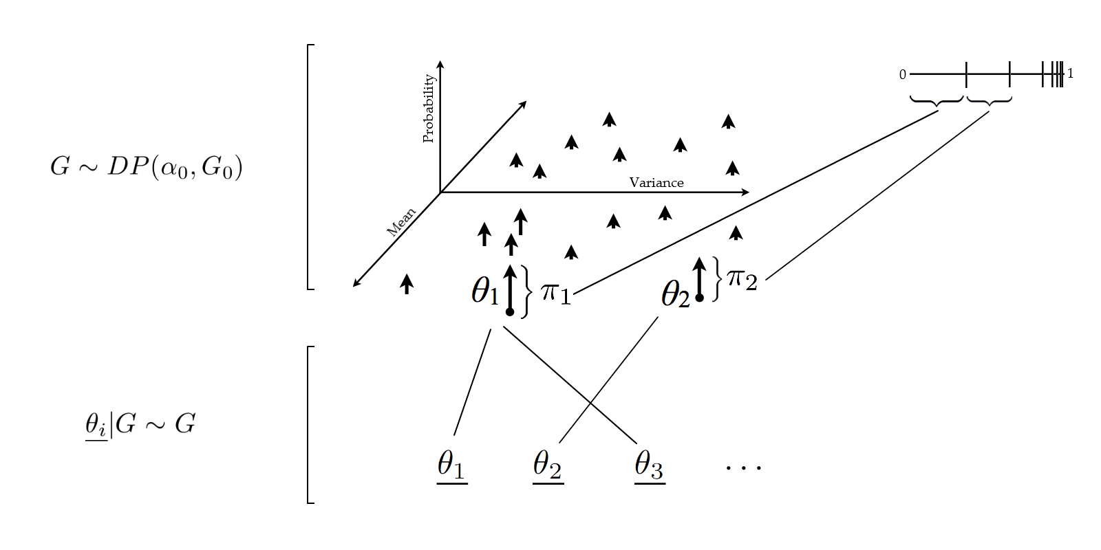
Since the realization of a DP is a probability distribution, we can sample from this realization! Let us call these samples from the DP sample $\underline{\theta_1}, \underline{\theta_2}, \dots$

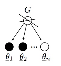
\begin{eqnarray} G & \sim & \DP \\ \underline{\theta_i} | G & \sim & G \end{eqnarray}

Preliminary observation: If I sample twice from an atomic distribution, there is a positive probability that I get two identical copies of the same point (an atomic measure $\mu$ is one that assign a positive mass to a point, i.e. there is an $x$ such that $\mu(\{x\}) > 0$). This phenomenon does not occur with non-atomic distribution (with probability one).

The realizations from the random variables $\underline{\theta_i}$ live in the same space $\Omega$ as those from $\theta_i$, but $\underline{\theta}$ and $\theta$ have important differences:

• The list $\underline{\theta_1}, \underline{\theta_2}, \dots$ will have duplicates with probability one (why?), while the list $\theta_1, \theta_2, \dots$ generally does not contain duplicates (as long as $G_0$ is non-atomic, which we will assume today).
• Each value taken by a $\underline{\theta_i}$ corresponds to a value taken by a $\theta$, but not vice-versa.

To differentiate the two, I will use the following terminology:

• Type: the variables $\theta_i$
• Token: the variables $\underline{\theta_i}$

Question: How can we simulate four tokens, $\underline{\theta_1}, \dots, \underline{\theta_4}$?

1. Hard way: use the stick breaking representation to simulate all the types and their probabilities. This gives us a realization of the random probability measure $G$. Then, sample four times from $G$.
2. Easier way: sample $\underline{\theta_1}, \dots, \underline{\theta_4}$ from their marginal distribution directly. This is done via the Chinese Restaurant Process (CRP).

Let us look at this second method. Again, we will focus on the algorithmic picture, and cover the theory after you have implemented these algorithms.

The first idea is to break the marginal $(\underline{\theta_1}, \dots, \underline{\theta_4})$ into sequential decisions. This is done using the chain rule:

1. Sample $\underline{\theta_1}$, then,
2. Sample $\underline{\theta_2}|\underline{\theta_1}$,
3. etc.,
4. Until $\underline{\theta_4}|(\underline{\theta_1}, \underline{\theta_2}, \underline{\theta_3})$.

The first step is easy: just sample from $G_0$! For the other steps, we will need to keep track of token multiplicities. We organize the tokens $\underline{\theta_i}$ into groups, where two tokens are in the same group if and only if they picked the same type. Each group is called a table, the points in this group are called customers, and the value shared by each table is its dish.

Once we have these data structures, the conditional steps 2-4 can be sampled easily using the following decision diagram:

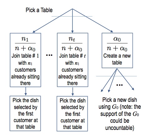
Following our example, say that the first 3 customers have been seated at 2 tables, with customers 1 and 3 at one table, and customer 2 at another. When customer 4 enters, the probability that the new customer joins one of the existing tables or creates an empty table can be visualized with the following diagram:

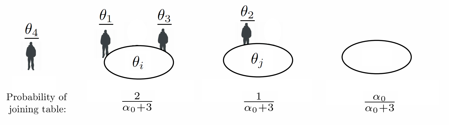
Formally:

\begin{eqnarray}\label{eq:crp} \P(\underline{\theta_{n+1}} \in A | \underline{\theta_{1}}, \dots, \underline{\theta_{n}}) = \frac{\alpha_0}{\alpha_0 + n} G_0(A) + \frac{1}{\alpha_0 + n} \sum_{i = 1}^n \1(\underline{\theta_{i}} \in A). \end{eqnarray}

Clustering/partition view: This generative story suggests another way of simulating the tokens:

1. Generate a partition of the data points (each block is a cluster)
2. Once this is done, sample one dish for each table independently from $G_0$.

By a slight abuse of notation, we will also call and denote the distribution on the partition the CRP. It will be clear from the context if the input of the $\CRP$ is a partition or a product space $\Omega \times \dots \times \Omega$.

Important exercise: Exchangeability. We claim that for any permutation $\sigma : \{1, \dots, n\} \to \{1, \dots, n\}$, we have:

\begin{eqnarray} (\underline{\theta_1}, \dots, \underline{\theta_n}) \deq (\underline{\theta_{\sigma(1)}}, \dots, \underline{\theta_{\sigma(n)}}) \end{eqnarray}

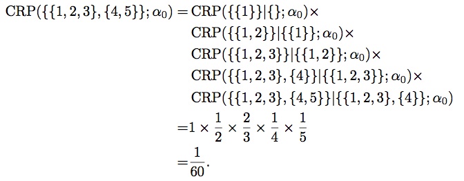
You can convince yourself with the following small example, where we compute a joint probability of observing the partition $\{\{1,2,3\},\{4,5\}\}$ with two different orders. First, with the order $1 \to 2 \to 3 \to 4 \to 5$, and $\alpha_0 = 1$:

Then, with the order $4 \to 5 \to 3 \to 2 \to 1$, we get:

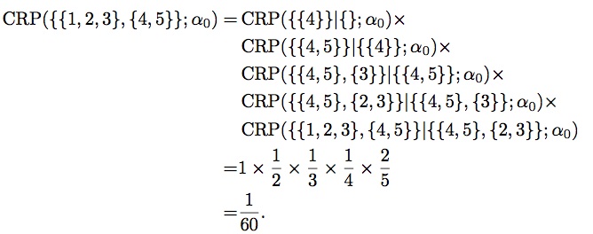
The product of these CRPs is called Ewens's sampling formula.

Dirichlet Process Mixture model

• In many applications, the observations in one cluster component are not all identical!
• This motivates the Dirichlet Process Mixture (DPM) model

A DPM is specified by:

• A likelihood model with density $\ell(x|\theta)$ over each individual observation (a weight). For example, a normal distribution (a bit broken since weights are positive, but should suffice for the purpose of exposition).
• A conjugate base measure, $G_0$, with density $p(\theta)$. As before, $\theta$ is an ordered pair containing a real number (modelling a sub-population mean) and a positive real number (modelling a sub-population variance (or equivalently, precision, the inverse of the variance)). A normal-inverse-gamma distribution is an example of such a prior.
• Some hyper-parameters for this parametric prior, as well as a hyper-parameter $\alpha_0$ for the Dirichlet prior.

To simulate a dataset, use the following steps:

1. Break a stick $\pi$ according to the algorithm covered in the previous section.
2. Simulate an infinite sequence $(\theta_1, \theta_2, \dots)$ of iid normal-inverse-gamma random variables. The first one corresponds to the first stick segment, the second, to the second stick segment, etc.
3. For each datapoint $i$:
   1. Throw a dart on the stick, use this random stick index $Z_i$. Grab the corresponding parameter $\theta_{Z_i}$.
   2. Simulate a new datapoint $X_i$ according to $\ell(\cdot | \theta_{Z_i})$.

This algorithmic description has the following graphical model representation (for details on the plate notation see the wiki page).

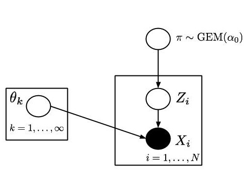
Equivalently:

1. Sample $(\underline{\theta_1}, \dots, \underline{\theta_n})$ from the CRP (where $n$ is the number of data points).
2. Simulate $X_i$ according to $\ell(\cdot | \underline{\theta_i})$.

Posterior simulation with MCMC

Important concept: Rao-Blackwellization.

• Reduce state space in which we do MCMC.
• Synonyms: collapsing, marginalization.
• Opposite of auxiliary variables, which enlarge (augment) the space.
• Rough comparison (not always true, i.e. the classical Rao-Blackwell does not always apply):
  • Rao-Blackwellization typically makes each MCMC iteration more expensive, but reduce the number of MCMC iterations required to get a certain accuracy of the MC averages
  • Auxiliary variables typically go the other way around.
  • Both can be combined (enlarging some aspects and collapsing others).

Formally:

• Let $s : \Xscr \to \Yscr$ be a map that simplifies the original state space $\Xscr$ of the MCMC into a reduced state space $\Yscr$.
• From the original target distribution $\pi$, build a new target distribution $\pi_\star$ defined as follows: for any $A \subset \Yscr$, let $\pi_\star(A) = \pi(s^{-1}(A))$. When we have densities, this gives us a density $\pi_\star(y) = \int_{x:s(x) = y} \pi(x) \ud x$ (assuming $s$ is non pathological).
• Now, design a proposal $q$ on the simplified space $\Yscr$ instead of $\Xscr$.
• Challenge: the MH ratio will involve $\pi_\star$, and therefore the integral needs to be solved analytically (other options??)

Examples:

• $x = (x_1, x_2)$, and $s_1(x) = x_1$.
• $v = (\pi_{1:\infty}, z_{1:n})$ and $s_2(v) = $ partition $\rho(v)$ of the samples $\underline{\theta_{1:n}}$ from the DP.
• $w = (\rho, \theta_{1:\infty})$ and $s_3(w) = \rho$.

Rao-Blackwellization in DPMs: with Dirichlet process priors (and Pitman-Yor priors):

1. You can always compute $\pi_\star(\rho) = \pi(s_2^{-1}(\rho))$ using Ewen's sampling formula (see the exercise above).
2. Moreover, if the parametric family $\ell$ is conjugate with $G_0$, we can also compute $\pi_{\star\star}(\rho) = \pi(s_3^{-1}(\rho))$, using formula (20) from lecture 2. This is called the collapsed sampler, as all the continuous variables have been marginalized.

Today: let us assume only (1) above, i.e. we have a likelihood $\ell$ which may not have a tractable conjugacy relationship with $G_0$.

State space:

• $\rho$ (i.e. we marginalize/simplify $\pi_{1:\infty}, z_{1:n}$ into $\rho$
• One parameter $\theta$ for each table, denoted $\theta_1, \dots, \theta_K$ (block in $\rho$). Note that $K$ is random, so the state space is a union of spaces of different dimensionalities.

MCMC moves:

1. Keep $\rho$ fixed, propose a change to one or several $\theta_k$, accept-reject using the standard MH ratio.
2. Take one customer out of the restaurant. Let $K_-$ be the number of non-empty tables after removing this customer ($K_-$ could be either the same as $K$, or $K-1$ if the customer was sitting by themselves). We will keep the parameters of these tables fixed. Propose a new table, out of: either an existing non-empty table, or a new table. Overall, the number of table $K'$ after the move can be either $K-1$, $K$, or $K+1$.

Note: move (2) can change the dimensionality of the space. How to approach this can be viewed through the lenses of RJMCMC:

• Add a temporary auxiliary variable $\theta^\star \sim G_0$
  • If the customer was sitting by themselves, augment the state space before the move,
  • Otherwise, augment the state space after the move
• As with the parameters $\lambda$ in the example of lecture 11, the Jacobian is one.

Details: assignment 2