While you start familiarizing yourself with java in preparation for the third exercise, in this exercise we will explore the basics of a simple language specialized to Bayesian inference called JAGS.

JAGS (or similar languages, such as Stan and WinBugs) and Java (or similar languages, such as C++, C# or Go) form a good combo for approaching Bayesian inference problems: the former for small problem and prototyping, and the latter for large scale and non-standard models.

Resources for this assignment

Optional readings

Start by familiarizing yourself with the main features of the JAGS modelling language. See the manual, especially 2.1, 2.2, 2.4, 2.5, 3, and have a quick look at 5, 6. If there are any questions, I will devote some time on Monday for Q&A.

Logistics

You should hand-in the CODA files produced by the MCMC run (see below), archived at the root of a zip file. Some questions may also require a pdf containing a plot and/or some comments and analysis. Use the same file naming convention as for the previous assignment.

You will have two options for solving this exercise:

• Use a web-based tool designed for this course, where you edit the model online and the code is executed on Amazon EC2 (see instructions below).
• Install JAGS locally (open source software available at http://mcmc-jags.sourceforge.net).

Web-based JAGS

1. Access this URL. Use chrome with a large window size if possible.
   • Username: your student number
   • Password: your student number
2. Click on the file on the left that you want to edit.
3. Write down the model in clustering.txt and the script controlling the number of iterations, variables to monitor, etc., in clustering.jags WARNING: make sure to press commit regularly and before switching files to edit.
4. To run:
   • you need to select the jags script you want to run.
   • click on clustering.jags and then:
   • click on the star '*' located besides the filename.
   • click on Run; this may take some time
   • once the execution is complete, you can press Download to get the output in a zip file. There will also be a textfile within the zip folder that provides some detail on the job run.

Updates on technical issues. My apologies for the glitches, but we will be working hard resolving any issue in a timely manner.

• Note: we are currently (Jan 18, 15:00) in the process of resolving a technical issue with running JAGS on the server. This should be resolved shortly. Problem resolved: if you see the message 'undefined' in the job window, just ignore it and download the output file; the correct output should be in there.
• There is currently a problem with the data for question 2 (Jan 19, 9:00). The corrected data will be redeployed shortly. You can get started anyways, but will have to wait a few hours before running your code.This issue is now resolved as well.

Skeleton files

Please use these skeleton files that contain some initial setup for answering the questions:

• Question 1
• Question 2
• Question 3

Reading CODA files

Whether you use the web-based tool or a local install, JAGS uses the CODA format to store samples extracted from an MCMC run. You can use the R libraries coda and mcmcplots to interpret a CODA file. For example, you can do the following to construct density estimates from an MCMC output stored in CODAchain1.txt and CODAindex.txt of the working directory:

library(coda)

pdf('analysis1.pdf')
res = read.coda("CODAchain1.txt", "CODAindex.txt")
plot(res)

dev.off()

Misc

Some potential traps:

• JAGS can have problems with observing deterministic nodes. You can always put a peaked normal around the value to sidestep that issue.
• While the syntax of R and JAGS are generally fairly similar, note one important difference: JAGS uses a precision parameter for the spread of normal distributions (the precision is the inverse of the variance), while R uses the standard deviation parameterization.

Question 1: Truncated DP posterior simulation in JAGS

Context

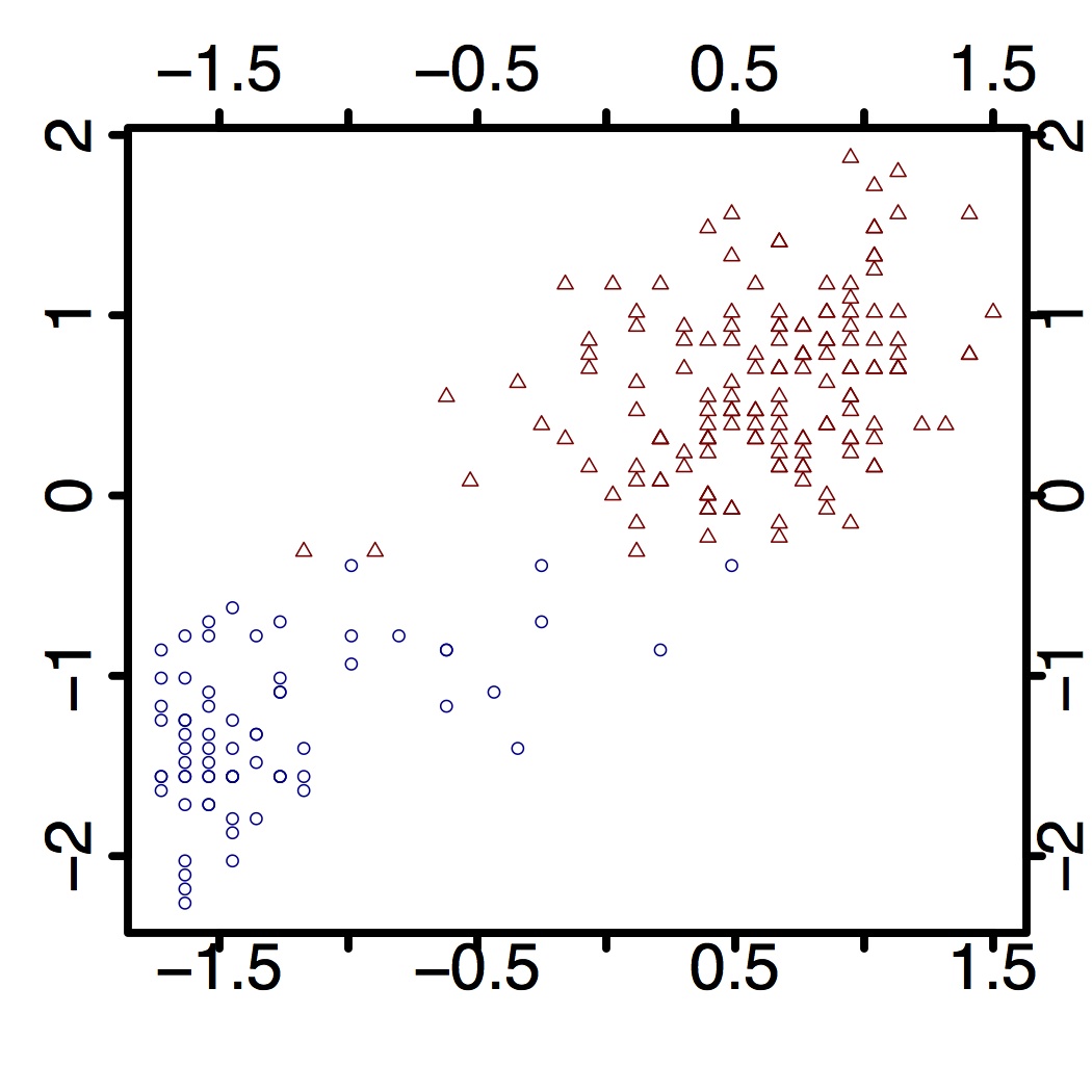In this question, you will use a truncated DP model to analyze the classical Old Faithful Geyser Data. The normalized version can be downloaded here. (side question: why do you think normalization useful in this context?)

Goal

The dataset contains a collection of pairs. Each pair contains an eruption time in minutes, a a waiting time to the next eruption. Note that we have held-out some values. The goal of this exercise will be to find the posterior distributions of the missing values via a truncated DP (lecture of Jan 15). Your answers should therefore consists in two file: a zip with the CODA samples, and a pdf containing density estimates of the approximate posteriors.

The model should have the following characteristics:

• a truncation $K = 5$
• $\alpha_0 = 10$, and
• a normal likelihood model with priors of your choice (note that conjugacy is not required here)

Question 2: A simple dead reckoning problem

Context

This question is inspired by a mammal tracking application recently presented a department seminar. The problem consists in a vastly simplified dead reckoning problem. Suppose we have a marine mammal tagged with a tracking device measuring GPS locations and acceleration. The GPS can give accurate, absolute positions, but when the animal dives, only the accelerometer is operational, giving noisy acceleration estimates.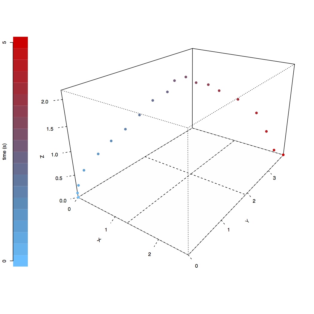

The objective is to reconstruct a trajectory given only its end-points and noisy intermediate accelerations. At the same time, we want to assess how reliable these estimates are.

Goal

The true trajectory (number of time steps=20) is shown in the figure on the right (where the $z$ axis is the depth), but note that your algorithm should only use the endpoints of this strategy. Your goal is to approximate the posterior density of the depth at time step 3, 10, and 19.

We will use the following simple kinetics model (see the the file located here for actual values of the variables used below):

• we ignore friction and gravity (!)
• we treat acceleration as instantaneous pulses, one at each point in the discretization, independently and normally distributed on each axis (with mean and sd given by true.accel.mean and true.accel.sd)
• we only observed a noisy version of each of the accelerations, assumed to be normally distributed around the truth, with sd given by accel.error.sd
• the time interval between time discretization grid points is assumed to be deltat
• only the initial position, true.pos[1,], initial velocity, true.velo[1,], and final position, true.pos[len,] are observed.

Your answers should consists in two file: a zip with the CODA samples, and a pdf containing density estimates of the posterior depths at time step 3, 10 and 19. Interpret and comment on whether these seem reasonable.

Optional question 3

In this question, you will build a simple hierarchical model to see how it can decrease the effect of hyper-parameters.

The data you will analyze consists in character n-gram counts extracted from two Austronesian languages, Iranun and Phan Rang Cham. The processed data can be downloaded here. The list named target contains counts for characters found in a small Iranun dataset (each column represent a character type, 29 types and 68 Iranun characters tokens). The goal is to estimate the population frequencies from these counts.

• Build a first Dirichlet multinomial model to infer these population frequencies. Try two values for the hyperpameters of the $\Dir(\alpha_1, \alpha_2, \dots, \alpha_{29})$, namely $\alpha = \alpha_i = 1$ and $\alpha = 0.1$ and see if the inferred posteriors qualitatively differ.
• Now, use the data from the related language, Phan Rang Cham, to improve your estimate. The data is in the vector related and contains 585 tokens organized into the same 29 types. Use a hierarchical Bayesian model containing two levels of Dirichlet distributions. Assess qualitatively the hyper-parameters sensitivity with this new model.
• The data also contains the union of both datasets, union, if you want to compare to the naive union-of-datasets approach.