Instructor: Alexandre Bouchard-Côté

Editor: Vincenzo Coia

Plan

Bayesian non-parametrics is a major area of application of stochastic processes in statistics, so we will devote the first few weeks on the topic. But before, let us review some concepts from parametric Bayesian statistics that will be useful in transitioning towards the non-parametric setup.

Overview of some useful concepts from Bayesian statistics

Consider the following generic statistical problem:

• we observe $x \in \Xscr$, we have a model of how this observation came to be in terms of some unknown quantities $z \in \Zscr$,
• and we want to make some decision (for example, reconstructing some of the unknown quantities, or forecasting future observations, etc).

More generally, we want to devise a decision-making strategy, which we formalize as an estimator: a function of the observation, $\delta(x)$.

We want this estimator to be as "good" as possible. Under a certain criterion of goodness, we will see that the Bayesian framework provides a principled and systematic way of specifying a "best" estimator.

Bayes estimators

Here is a very frequent misconception about the Bayesian framework that we will try to correct: "Bayesian methods consist of computing the posterior distribution and returning the point with the highest posterior density (1)." Other variants: "Bayesian methods consist of returning the posterior expectation of the parameters (2)."

While the posterior distribution is always involved in Bayesian methods, and that this posterior is sometimes used as in (1, 2) above, in other cases the Bayesian framework will prescribe other uses of the posterior.

How to use the posterior in general under the Bayesian framework is specified by the Bayes estimator.

In full generality, approaching a problem in a Bayesian way consists of:

1. specifying two quantities:
   • A model: which is simply a joint probability distribution $\P$ over the known and unknown quantities, modelled as random variables $X$ and $Z$ respectively.
   • A goal: specified by a set of actions $\Ascr$ (each action $a$ could be predictions, a decision, etc), together with a loss function $L(a, z)$, which specifies a cost incurred for picking action $a$ when the true state of the world is $z$. An important example, when $\Ascr$ coincides with the space of realization of $Z$, is $L(z', z) = (z - z')^2$, the squared loss.
2. selecting an estimator $\delta$ by minimizing the integrated risk, $\E[L(\delta(X), Z)]$.

Solving an optimization problem over a space of estimators seems quite abstract and hard to implement. Fortunately, it is possible to rewrite this optimization problem over the space of actions $\Ascr$. In other words, there is one general recipe for solving the above minimization problem:

Proposition: The estimator $\delta^*$, defined with the equation below, minimizes the integrated risk: \begin{eqnarray}\label{eq:bayes} \delta^*(X) = \argmin \{ \E[L(a, Z) | X] : a \in \Ascr \} \end{eqnarray}

This estimator $\delta^*$ is called a Bayes estimator.

This means that given a model and a goal, the Bayesian framework provides in principle a recipe for constructing an estimator.

Moreover, if the loss is strictly convex, the Bayes estimator is unique. See Robert 2007. In other words, under strictly convex losses, the Bayesian framework endows the space of estimators with a total order.

However, the computation required to implement this recipe may be considerable. This explains why computational statistics plays a large role in Bayesian statistics and in this course.

---

Optional exercise: If you have not seen this material before, show that in the special case where $L$ is the squared loss, one can compute a simple expression for the minimizer, which is simply $\delta^*(X) = \E[Z|X]$.

For other losses finding such an expression may or may not be possible. We will talk about approximation strategies for the latter case later in this course.

---

Note that other criteria certainly exist for selecting estimators, in particular frequentist criteria. Some of these criteria, such as admissibility, do not create a total order on the estimator (even under strictly convex losses), they only provide a partial order. Moreover, since the Bayes estimator can be shown to be non-suboptimal under this criterion as well (in other words, admissible)

Of course, these nice properties assume that the model is a true representation of the world (a well-specified model), a condition that is almost always false.

This provides a motivation for creating richer models that are more faithful to reality. In particular, models of adaptive complexity, that become progressively complex as more data become available. These models are called non-parametric (more formal definition below). As alluded last lecture, stochastic processes provide a formidable tool for constructing these non-parametric models.

Well-specified Bayesian models exist, but can force us to be non-parametric

Let us make the discussion on de Finetti from last week more formal.

Recall: A finite sequence of random variables $(X_1, \dots, X_n)$ is exchangeable if for any permutation $\sigma : \{1, \dots, n\} \to \{1, \dots, n\}$, we have:

\begin{eqnarray} ({X_1}, \dots, {X_n}) \deq ({X_{\sigma(1)}}, \dots, {X_{\sigma(n)}}). \end{eqnarray}

Extension: A countably infinite sequence of random variable $(X_1, X_2, \dots)$ is (infinitely) exchangeable if all finite sub-sequence $(X_{k_1}, \dots, X_{k_n})$ are exchangeable.

---

Example: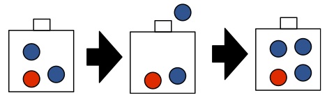

In the first exercise, you will show that any finite or infinite list of tokens sampled from a CRP is exchangeable. Here is a consequence:

• pick $G_0$ to be a discrete measure on two colors (red and blue):
  • red with probability $2/3$, and
  • blue with probability $1/3$ (we assumed last time that $G_0$ was non-atomic, but the theory extends easily to atomic $G_0$, the only difference is that two different tables can pick the same dish type).
• Interpretation as an urn model?

This means that the probability of observing the sequence of colors

red, red, red, red, red, red, blue, blue

is the same as the probability of observing the sequence

blue, blue, red , red , red , red, red, red

---

Theorem: De Finetti (simple version): If $(X_1, X_2, \dots)$ is an exchangeable sequence of binary random variables, $X_i : \Omega' \to \{0,1\}$ then there exists a random variable $Z : \Omega' \to [0, 1]$ such that $X_i | Z \sim \Bern(Z)$.

In other words, if all we are modelling is a sequence of exchangeable binary random variables, we do not need a non-parametric model. On the other hand, if the $X_i$ are real, the situation is different:

Theorem: De Finetti (more general version, see Kallenberg, 2005, Chapter 1.1): If $(X_1, X_2, \dots)$ is an exchangeable sequence of real-valued random variables, the there exists a random measure $G : \Omega' \to (\sa_{\Omega} \to [0,1])$ such that $X_i | G \sim G$.

Note that this random measure $G$ is not necessarily Dirichlet-Process distributed. Here is a counter-example, the Pitman-Yor process, which has the same structure as the CRP, with the following amendments:

• We boost the probability of creating a new table by $T_n \cdot d$, where:
  • $T_n$ is the current number of occupied tables (before seating a new customer)
  • $d$ is a hyper-parameter called a discount such that $0 \le d < 1$ (note that we also gain some extra freedom on $\alpha_0$, now it can be "slightly negative", namely $\alpha_0 > -d$).
• For each currently occupied table, we reduce the probability of joining that table by the constant $d$.

Optional exercise: this is still exchangeable, yet for $d \neq 0$, this is not the marginal of a Dirichlet process (in other words, this does not have the distribution of a sample of a sampled Dirichlet process).

Bayesian estimation in parametric families

Many non-parametric models are built by composing a random number of parametric models (DP by themselves would be limited since it would predict duplicates in the observations, which we may not want). Therefore, it is worth spending some time on parametric models initially. This will help clarify the formal definition of parametric vs. non-parametric at the same time.

Formally, a parametric Bayesian model contains two ingredients:

1. A collection of densities over the observations $\Xscr$, indexed by the space of unknowns $\Zscr$. These densities are called likelihoods, $\Lscr = \{\ell(x | z) : z\in\Zscr\}$. The parametric assumption simply means that the collection is smoothly indexed by a subset of an Euclidean space, $\Zscr \subset \RR^k$ for some fixed integer $k$.
2. A prior density $p$ on $Z$._{Note: the random variables $X, Z$ are not necessarily continuous, so the densities $\ell$ and $p$ are defined with respect to some arbitrary (but fixed and known) reference measures. Since they do not play a central role in the theory, we will keep these reference measures anonymous, writing $\ud x, \ud z$ for integration with respect to these variables.}

---

Example: Consider a multinomial (categorical) likelihood model over three categories. This means that each individual observation $x_i$ is a point from a finite set of $k = 3$ objects, and the full dataset is: $ x = (x_1, \dots, x_n), x_i \in \{\textrm{category 1, category 2, category 3}\}$. The parameter consists of three numbers $z = (z_1, z_2, z_3)$ that sum to one. This is a subset of $\RR^3$, therefore this is a parametric model. The value of the likelihood is given by:

\begin{eqnarray} \ell(x | z) = z_1^{n_1(x)} z_2^{n_2(x)} z_3^{n_3(x)}, \end{eqnarray}

where $n_k(z)$ returns the number of times category $k$ was picked among the $n$ observations $x= (x_1, \dots, x_n)$ (since the likelihood only depends on the function $n = (n_1, n_2, n_3)$, we say that $n$ is a sufficient statistic). As we have discussed last week, a suitable prior on $z$ is given by picking a Dirichlet distribution,

\begin{eqnarray} p(z) = z_1^{\alpha_1} z_2^{\alpha_2} z_3^{\alpha_3}, \end{eqnarray}

---

In order to evaluate our objective function, Equation~(\ref{eq:bayes}), we need to compute posterior expectations of the form $\E[\phi(Z)|X]$, where $\phi(z) = L(a,z)$ for some $a$ that we consider fixed for now.

Let us denote the posterior density by $p(z|x)$. We need to compute:

\begin{eqnarray}\label{eq:posterior} \int \phi(z) p(z|x) \ud z. \end{eqnarray}

By Bayes rule, this posterior density is proportional to the joint density (up to null sets), in other words, proportional to a prior times a likelihood (chain rule):

\begin{eqnarray} p(z|x) \propto p(z) \ell(x|z), \end{eqnarray}

with the following normalization for the right-hand side:

\begin{eqnarray}\label{eq:marginal} m(x) = \int p(z) \ell(x|z) \ud z. \end{eqnarray}

This normalization, denoted by $m(x)$, is called the marginal likelihood or evidence. If the observations $x$ are discrete, this corresponds to the probability of the observed dataset under the model (given the number of observations). For this reason, the evidence plays an important role in Bayesian model selection.

The integrals in Equations~(\ref{eq:posterior}, \ref{eq:marginal}) constitute one of the main challenge in Bayesian inference. We will discuss two approaches to solve these integrals in this course.

• Approximating the integral via Monte Carlo methods (next week)
• Picking the prior and likelihood so that analytic computations are possible (described in the next section).

Conjugacy in parametric families

Let us say that we are given a fixed likelihood model $\Lscr$. Our strategy to ensure tractable expressions in Equations~(\ref{eq:posterior}, \ref{eq:marginal}) consists in constructing a family of distributions over $z$, $\Cscr = \{p_h\}$ (where $h$ is an index called a hyper-parameter), such that:

1. The prior density is in this family: $p = p_{h_0} \in \Cscr$
2. More generally, given any observed dataset $x$, the posterior density should be a member of the conjugate family: $p(z|x) = p_{h'}(z) \in \Cscr$ for some updated hyper-parameters $h'$.

Finding a collection that satisfies these two conditions is easy. For example, if $\Lscr$ is an exponential family with $k$-dimensional parameters, it is always possible to find a conjugate family with $(k+1)$-dimensional parameters (see this hand-out). Note also that trivially, the class of all distributions is conjugate to any likelihood model.

But in order for the conjugate approach to be computationally feasible, we should also ensure that:

• Each member $p_h$ of the family should be tractable, in particular we should have an efficient algorithm for computing the normalization constant of arbitrary members.
• We should also have an efficient algorithm for finding updated parameters $h'$, as a function of the observed data $x$ and prior hyper-parameters $h_0$, $h' = u(x, h_0)$.

---

Example (continued): the Dirichlet distributions with hyperparameters $h = \alpha$ are conjugate to the multinomial likelihood. Moreover, the Dirichlet-multinomial model has the two nice computational tractability properties listed above.

Recall that for any hyper-parameter vector $h = \alpha$, a distribution on the simplex proportional to $z_1^{\alpha_1} z_2^{\alpha_2} z_3^{\alpha_3}$ has a known normalization $N(\alpha)$, namely

\begin{eqnarray}\label{eq:dir-norm} p_\alpha(z) & = & \frac{z_1^{\alpha_1} z_2^{\alpha_2} z_3^{\alpha_3}}{N(\alpha)} \\ N(\alpha) & = & \frac{\Gamma(\alpha_1) \Gamma(\alpha_2) \Gamma(\alpha_3)}{\Gamma(\alpha_1 + \alpha_2 + \alpha_3)}. \end{eqnarray}

Now let us look at the form of the posterior (up to normalization):

\begin{eqnarray}\label{eq:dir-prop} p(z | x) & \propto & p_\alpha(z) \ell(x | z) \\ & \propto & z_1^{n_1(x) + \alpha_1} z_2^{n_2(x) + \alpha_2} z_3^{n_3(x) + \alpha_3}. \end{eqnarray}

To conclude, we use the simple but extremely useful fact that if two densities are proportional (in this case, Equation~(\ref{eq:dir-norm}) and (\ref{eq:dir-prop})), then they are equal (up to null sets). By Equation~(\ref{eq:dir-norm}), we can therefore conclude that the hyper-parameters update is given by $u(x, \alpha) = \alpha + n(x)$.

---

Another important example of a conjugate family is the normal-inverse-gamma distribution. Please read this article.

One final note that we will use later: tractable conjugacy also gives us a way of computing the evidence $m(x)$. This is done by rearranging Bayes rule:

\begin{eqnarray} m(x) & = & \frac{p_{h}(z) \ell(x | z)}{p(z | x)} \\ & = & \frac{p_{h}(z) \ell(x | z)}{p_{u(x, h)}(z)}. \end{eqnarray}

Since this is true for all $z$, we can pick an arbitrary $z_0$, and evaluate each component of the right-hand side by assumption.

Hierarchical models

Since conjugacy leads us to consider families of priors indexed by a hyper-parameter $h$, this begs the question of how to pick $h$. Note that both $m_h(x)$ and $p_h(z | x)$ implicitly depend on $h$. Here are some guidelines for approaching this question:

1. One can maximize $m_h(x)$ over $h$, an approach called empirical Bayes. Note however that this does not fit the Bayesian framework (despite its name).
2. If the dataset is moderate to large, one can test a range of reasonable values for $h$ (a range obtained for example from discussion with a domain expert); if the risk of the action selected by the Bayes estimator is not affected (or not affected too much), one can side-step this issue and pick arbitrarily from the set of reasonable values.
3. If it is an option, one can collect more data from the same population. Under regularity conditions, the effect of the prior can be decreased arbitrarily (this follows from the celebrated Bernstein-von Mises theorem, see van der Vaart, p.140).
4. If we only have access to other datasets that are related (in the sense that they have the same type of latent space $\Zscr$), but potentially from different populations, we can still exploit them using a hierarchical Bayesian model, described next.

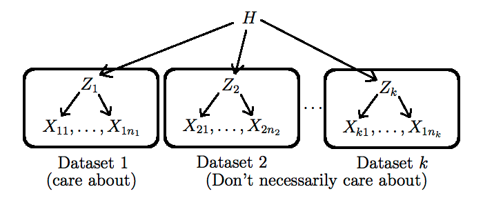
Hierarchical Bayesian models are conceptually simple:

1. We create distinct, exchangeable latent variables $Z_j$, one for each related dataset $X_j$
2. We make the hyper-parameter $h$ be the realization of a random variable $H$. This allows the dataset to originate from different populations.
3. We force all $Z_j$ to share this one hyper-parameter. This step is crucial as it allows information to flow between the datasets.

One still has to pick a new prior $p^*$ on $H$, and to go again through steps 1-4 above, but this time with more data incorporated. Note that this process can be iterated as long as there is some form of known hierarchical structure in the data (as a concrete example of a type of dataset that has this property, see this non-parametric Bayesian approach to $n$-gram modelling: Teh, 2006). More complicated techniques are needed when the hierarchical structure is unknown (we will talk about two of these techniques later in this course, namely hierarchical clustering and phylogenetics).

The cost of taking the hierarchical Bayes route is that it generally requires resorting to Monte Carlo approximation, even if the initial model is conjugate.

Supplementary references and notes

Robert, C. (2007) The Bayesian Choice. An excellent textbook, especially for the theoretically foundations of Bayesian statistics. Also covers many practical topics. Most relevant to this course are chapters 2, 3.1-3.3, 4.1-4.2.

van der Vaart, A.W. (1998) Asymptotic Statistics. Chapter 10 contains a formal treatment of the asymptotic properties of parametric Bayesian procedures. Note that a different treatment is needed for non-parametric Bayesian procedures. We will come back to this issue next week.