Lecture 4: Dirichlet process: inference, properties and extensions
Instructor: Alexandre Bouchard-Côté
Editor: Sean Jewell
Composing many parametric models into a larger, non-parametric model
Based on these notes from the previous time I taught the course.
Dirichlet process mixture model
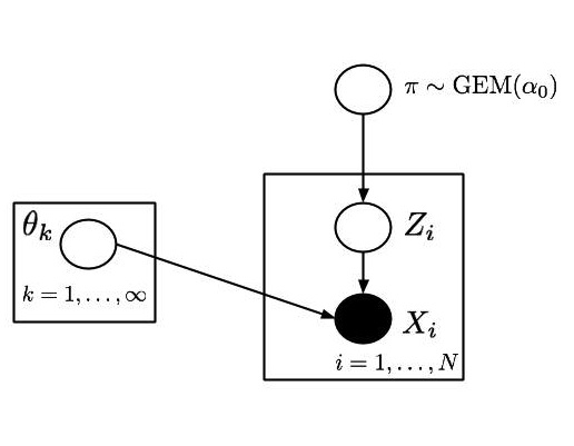
We can now integrate these new concepts to make our picture of Bayesian non-parametric mixture models more precise. Let us start with a model based on the stick breaking representation. Later, we will connect it to the CRP representation.
We pick:
- A likelihood model with density $\ell(x|\theta)$ over each individual observation (a weight). For example, a normal distribution (a bit broken since weights are positive, but should suffice for the purpose of exposition).
- A conjugate base measure, $G_0$, with density $p(\theta)$. As before, $\theta$ is an ordered pair containing a real number (modelling a sub-population mean) and a positive real number (modelling a sub-population variance (or equivalently, precision, the inverse of the variance)). A normal-inverse-gamma distribution is an example of such a prior.
- Some hyper-parameters for this parametric prior, as well as a hyper-parameter $\alpha_0$ for the Dirichlet prior.
To simulate a dataset, use the following steps:
- Break a stick $\pi$ according to the algorithm covered last time.
- Simulate an infinite sequence $(\theta_1, \theta_2, \dots)$ of iid normal-inverse-gamma random variables. The first one corresponds to the first stick segment, the second, to the second stick segment, etc.
- For each datapoint $i$:
- Throw a dart on the stick, use this random stick index $Z_i$. Grab the corresponding parameter $\theta_{Z_i}$.
- Simulate a new datapoint $X_i$ according to $\ell(\cdot | \theta_{Z_i})$.
This algorithmic description has the following graphical model representation (for details on the plate notation see the wiki page).
Truncated DPM posterior simulation
While forward simulation is easy, exact posterior simulation is computationally hard, as we will see later in this course. We will therefore need approximate posterior simulation. The good news is that we can show only one additional operation is required: computing the density of a realization of $\pi, Z, X$.
Depending on the situation, computing the density of a realization can be easy or hard. It is hard when there is a complicated set of outcomes that lead to the same realization. Fortunately, this is not the case here.
Another complication is that the space is infinite-dimensional, and taking an infinite product of densities is ill-behaved. We will see two elegant ways of resolving this shortly. For now, let us just truncate the DP: for some fixed $K$, set $\beta_K = 1$. This gives probability zero to the subsequent components. We can then express the joint distribution of $\pi, \theta, Z, X$ via the density:
\begin{eqnarray}\label{eq:joint} p(\pi, \theta, z, x) = \left(\prod_{k=1}^K \Beta(\beta_k(\pi); 1, \alpha_0) p(\theta_k) \right) \left( \prod_{i=1}^N \Mult(z_i; \pi) \ell(x_i | \theta_{z_i}) \right). \end{eqnarray}
Here $\beta_k(\pi)$ is a deterministic function that returns the $k-th$ beta random variable used in the stick breaking process given a broken stick $\pi$ (convince yourself that these beta variables can be recovered deterministically from $\pi$. There exists a one-to-one mapping between $\pi$ and $\beta$.)
Evaluation of Equation~(\ref{eq:joint}) is the main calculation needed to run a basic MCMC sampler for posterior simulation of a truncated DP.
Dish marginalization when conjugacy is available
Rao-Blackwellization: as we will see, it is often useful to marginalize some variables and to then define MCMC samplers on this smaller space (obtained through marginalization).
We will show it is possible to marginalize both $\pi$ and $\theta$. Today, we first consider marginalizing only $\theta$.
Example: Let us look at an example how this works:
- Suppose that in a small dataset of size three, the current state of the sampler is set as follows: the current table assignment $z$ consists of
- two datapoints at one table,
- and one datapoint alone at its table.
- Set the truncation level $K=4$.
Let us group the terms in the second parenthesis of Equation~(\ref{eq:joint}) by $\theta_k$:
\begin{eqnarray} p(\pi, \theta, z, x) & = & \left(\prod_{k=1}^K \Beta(\beta_k(\pi); 1, \alpha_0) \right) \left( \prod_{i=1}^N \Mult(z_i; \pi) \right) \\ & & \times \left( p(\theta_1) \ell(x_1 | \theta_1) \right) \\ & & \times \left( p(\theta_2) \ell(x_2 | \theta_2) \ell(x_3 | \theta_2) \right) \\ & & \times \left( p(\theta_3) \right) \\ & & \times \left( p(\theta_4) \right). \end{eqnarray}
To get the marginal over $(\pi, Z, X)$, we need to integrate over $\theta_1, \dots, \theta_4$. For tables with nobody sitting at them, we get factors of the form:
\begin{eqnarray} \int p(\theta_3) \ud \theta_3 = 1. \end{eqnarray}
For the occupied tables, we get a product of factors of the form:
\begin{eqnarray} \int p(\theta_2) \ell(x_2 | \theta_2) \ell(x_3 | \theta_2) \ud \theta_2. \end{eqnarray}
But this is just $m(x_2, x_3)$, which we can handle by conjugacy! Recall from last lecture:
\begin{eqnarray} m(x) & = & \frac{p_{h}(z) \ell(x | z)}{p(z | x)} \\ & = & \frac{p_{h}(z) \ell(x | z)}{p_{u(x, h)}(z)}. \end{eqnarray}
Here $x$ is a subset of the dataset, given by the subset of the points that share the same table.
Notation: Let us introduce some notation for the subset of people that share the same table.
- Note first that the assignments $z$ induce a partition $\part(z)$ of the customer indices (datapoint indices $\{1, 2, \dots, N\}$).
- Each block $B \in \part(z)$ then corresponds to the subset of indices of the customers sitting at a table.
- Finally, we will write $x_B$ for the subset of the observations themselves; for example in the above example $\part(z) = \{\{1\}, \{2,3\}\}$ and if $B = \{2, 3\}, x_B = (x_2, x_3)$.
This gives us:
\begin{eqnarray} \int p(\pi, \theta, z, x) \ud \theta & = & \left(\prod_{k=1}^K \Beta(\beta_k(\pi); 1, \alpha_0) \right) \left( \prod_{i=1}^N \Mult(z_i; \pi) \right) \times \prod_{B \in \part(z)} \left( \int p(\theta) \prod_{i\in B} \ell(x_i | \theta) \ud \theta \right) \\ & = &\left(\prod_{k=1}^K \Beta(\beta_k(\pi); 1, \alpha_0) \right) \left( \prod_{i=1}^N \Mult(z_i; \pi) \right) \times \prod_{B \in \part(z)} m(x_B) \end{eqnarray}
Stick marginalization using CRP
We will now push this marginalization further, marginalizing over both $\theta$ and $\pi$ this time. In fact, the only latent variable we will keep around is $\part(Z)$, the partition induced by the repeated DP sampling. This allows us to get rid of the truncation at the same time.
In order to formalize this idea, we will avoid the density notation and work with Lebesgue integrals with respect to measures. Let us denote the measure on sticks induced by the stick breaking process by $\gem$. Assume for simplicity that the observations are discrete.
We want to compute, for any partition $\part = \{B_1, \dots, B_K\}$ of $\{1, 2, \dots, N\}$:
\begin{eqnarray} \P(\part(Z) = \part, X = x) & = & \int \int \P(\part(Z) = \part|\pi) \left( \prod_{k=1}^K \prod_{i \in B_k} \ell(x_i | \theta_k) \right) G_0^\infty(\ud \theta) \gem(\ud \pi; \alpha_0) \\ & = & \label{eq:marg} \left( \int \P(Z = z|\pi) \gem(\ud \pi; \alpha_0) \right) \left( \int \left( \prod_{i=1}^N \ell( x_i | \theta_{z_i}) \right) G_0^\infty(\ud \theta) \right) \end{eqnarray}
We showed in the previous section how to compute the second parenthesis of Equation~(\ref{eq:marg}).
For the first parenthesis of the same equation, we need to compute the probability of observing a seating arrangement integrating over the stick lengths. We have discussed last lecture that this is given by the CRP (and we will explain why this is the case in the following section). Let us denote the probability of this seating arrangement (marginalizing over sticks) by $\CRP(\part(z))$. Recall that this probability can be computed by creating the partition one point at the time (in any order), multiplying conditional CRP probabilities.
Combining these two facts yields:
\begin{eqnarray} \P(\part(Z) = \part, X = x) & = & \label{eq:crp-joint} \CRP(\part(z); \alpha_0) \left( \prod_{B \in \part(z)} m(x_B) \right) \end{eqnarray}
Surprisingly, we managed to get rid of all continuous latent variables! So, in principle, we could compute the exact posterior probability $\P(Z = z | X = x)$ by summing over all partitions $\part$. In practice, the number of partitions is super-exponential, so this is not practical for large problems. As a result we use an approximation algorithm such as MCMC. But the explicit exact formula can be useful on tiny examples, in particular, for debugging approximation algorithms.
Theoretical properties of DPs
Let us look now at the theoretical justifications of some of the steps we took in the previous argument. First, we will need yet another characterization/definition of the DP.
FDDs of a DP
Consider the following thought experiment:
- Fix a partition of $\Omega$: $A_1, A_2, A_3$.
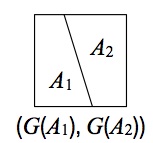
- Imagine that we simulate a realization of $G$.
- Let us look at $G(A_1)$. What is that? Just the sum of the heights of the sticks that fall in $A_1$.
- Do the same for $A_2, A_3$. We get a triplet of positive real numbers $(A_1, A_2, A_3)$.
- Now let's repeat the steps 2-4. We get a list of triplets. Let's ask the following question: what is the multivariate distribution of these triplets?
Equivalent definition of a Dirichlet Process: We say that $G : \Omega' \to (\sa_{\Omega} \to [0, 1])$ is distributed according to the Dirichlet process distribution, denoted $G \sim \DP(\alpha_0, G_0)$, if for all measurable partitions of $\Omega$, $(A_1, \dots, A_m)$, the FDDs are Dirichlet distributed: \begin{eqnarray}\label{eq:dp-marg} (G(A_1), \dots, G(A_m)) \sim \Dir(\alpha_0 G_0(A_1), \dots, \alpha_0 G_0(A_m)). \end{eqnarray}
Question: First, why is this declarative definition well-defined? In other words, why are we guaranteed that there exists a unique process that satisfies Equation~(\ref{eq:dp-marg})?
Answer: This follows from the Kolmogorov extension theorem. We will revisit this theorem later in more detail, but informally it says that if we can show that the marginal specified by Equation~(\ref{eq:dp-marg}) are consistent, then existence and uniqueness of a process is guaranteed by the Kolmogorov extension theorem.
The main step can be illustrated by this example:
Proposition: Let $(A_1, A_2)$ and $(B_1, B_2, B_3)$ be the following two measurable partitions of $\Omega$:
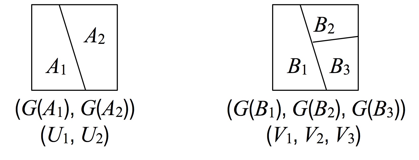
I.e. $A_1 = B_1$, and $(B_2, B_3)$ is a partition of $A_2$. Let $U_1, U_2$ and $V_1, V_2, V_3$ be the random variables as defined in the figure above ($U_1 = G(A)$, etc.). Then: $(U_1, U_2) \deq (V_1, V_2 + V_3)$, where the special equality symbol denotes equality in distribution.
In order to prove this, we use an important tool in the study of Dirichlet processes: gamma representation of Dirichlet distributions:
Lemma: If $Y_1, \dots, Y_K \sim \gammarv(\alpha_i, \theta)$ are independent, where $\alpha_i$ is a shape parameter and $\theta$ is the scale parameter, then: \begin{eqnarray} \left(\frac{Y_1}{\sum_k Y_k}, \dots, \frac{Y_K}{\sum_k Y_k}\right) \sim \dir(\alpha_1, \dots, \alpha_K). \end{eqnarray}
Proof: A standard change of variable problem. See the wikipedia page on the Dirichlet distribution and citations there-in.
We now turn to the proof of the proposition:
Proof: Let $\theta > 0$ be an arbitrary scale parameter, and $Y_i \sim \gammarv(\alpha_0 G_0(B_i), \theta)$ be independent. From the lemma: \begin{eqnarray} (V_1, V_2 + V_3) &\deq \left(\frac{Y_1}{\sum_k Y_k}, \frac{Y_2 + Y_3}{\sum_k Y_k}\right) \ &\deq \left(\frac{Y_1}{\sum_k Y_k}, \frac{Y'}{\sum_k Y_k}\right) \ &\deq (U_1, U_2), \end{eqnarray} where $Y' \sim \gammarv(G_0(B_2) + G_0(B_3), \theta) = \gammarv(G_0(A_2), \theta)$ by standard properties of Gamma random variables.
The full proof would consider any finite number of blocks, but follows the same argument. Therefore, we indeed have a stochastic process.
Formal connection between the CRP and process definitions
The key step to show this connection is to prove that the Dirichlet process is conjugate to multinomial sampling. This is done by lifting the argument that Dirichlet-multinomial is conjugage via Kolmogorov consistency.
Let $G\sim \dirp(\alpha_0, G_0)$.
Recall:
- since $G$ is a measure-valued random variable, we can sample random variables $\utheta$ from realizations of $G$, i.e. we define $\utheta$ by $\utheta | G \sim G$. Recall that the notation $\utheta | G \sim G$ means: for all bounded $h$, $\E[h(\utheta) | G] = \int h(x) G(\ud x) = \sum_{c=1}^\infty \pi_c h(\theta_c)$ for $\pi\sim\gem(\alpha_0)$ and $\theta_c \sim G_0$ independent.
- we are using the underscore to differentiate the random variables $\theta_i$ used in the stick breaking construction (types) from the samples $\utheta_i$ from the Dirichlet process (tokens).
- $\utheta = \theta_x$ for a random $x$ sampled from a multinomial distribution with parameters given by the sticks $x\sim\mult(\pi)$.Note that finite multinomial distributions over ${1, 2, \dots, K}$ can be extended to distributions over the infinite list ${1, 2, \dots}$, in which case they take as parameters an infinite list of non-negative real numbers that sum to one (e.g.: sticks from the stick breaking construction). We saw in the first exercise how to sample from such generalized multinomials in practice.
In this section we show that the Dirichlet process is conjugate in the following sense: $G | \utheta \sim \dirp(\alpha'_0, G'_0)$ for $\alpha'_0, G'_0$ defined below.
To prove this result, we first look at the posterior of the finite dimensional distributions:
Lemma: If $(B_1, \dots, B_K)$ is a measurable partition of $\Omega$, then: $$(G(B_1), \dots, G(B_K))|\utheta \sim \dir\big(\alpha_0G_0(B_1) + \delta_{{\utheta}}(B_1), \dots, \alpha_0G_0(B_K) + \delta_{{\utheta}}(B_K)\big).$$
Proof: Define the random variables $Z = (G(B_1), \dots, G(B_K))$ and $X = (\delta_{\utheta(1)}(B_1), \dots, \delta_{\utheta(1)}(B_K)$. We have: \begin{eqnarray} Z&\sim\dir(\alpha_0G_0(B_1) , \dots, \alpha_0G_0(B_K)) \ \quad X | Z &\sim \mult(Z). \end{eqnarray} The result follows by standard Dirichlet-multinomial conjugacy.
Since this result is true for all partitions, this means that the posterior is a Dirichlet process as well by the Kolmogorov consistency definition!
We can now obtain the parameters $\alpha'_0, G'_0$ of the updated Dirichlet process. To get $\alpha_0$, we take the sum of the parameters of any finite dimensional Dirichlet distribution, obtaining $\alpha'_0 = \alpha_0 + 1$. To get $G'_0$, we normalize the expression in the conclusion of the last lemma to get: \begin{eqnarray} G'_0 & = & \frac{\alpha_0}{\alpha_0 + 1}G_0 + \frac{1}{\alpha_0+1} \delta_{{\utheta}} \\ \alpha'_0 & = & \alpha_0 + 1. \end{eqnarray}
This formula can be generalized to the case of multiple observations, by applying it $n$ times:
Proposition: Suppose $G \sim \dirp(\alpha_0, G_0)$ and $\utheta_i | G \sim G$ for $i\in{1, \dots, n}$, iid given $G$. Then the posterior has the following distribution: \begin{eqnarray} G | \utheta_1, \dots, \utheta_n \sim \dirp\left(\alpha_0 + n, \frac{\alpha_0}{\alpha_0 + n} G_0 + \frac{1}{\alpha_0+n} \sum_{i=1}^n \delta_{{\utheta_i}}\right). \end{eqnarray}
Equivalence of stick breaking and process definitions
Refer to section 2.5 of these notes from the first time I taught the course.
Supplementary references and notes
Markov Chain Sampling Methods for Dirichlet Process Mixture Models Radford M. Neal Journal of Computational and Graphical Statistics , Vol. 9, No. 2 (Jun., 2000) , pp. 249-265
Gibbs Sampling Methods for Stick-Breaking Priors Hemant Ishwaran and Lancelot F. James Journal of the American Statistical Association , Vol. 96, No. 453 (Mar., 2001) , pp. 161-173