Instructor: Alexandre Bouchard-Côté

Editor: Fatemeh Dorri

Brief Overview

Based on slides I created the first time I taught this course: PDF.

What is a stochastic process? Stochastic process or random process is a collection of random (not necessarily independent) variables indexed by an arbitrary set $S$. This gets interesting when $S$ is uncountable.

Topic of this course: Why/when is it useful to have $S$ uncountable? How can we still do inference using our finite brains and computers?

Note: $S$ is not necessarily a subset of the real line!

Examples of stochastic processes:

Time series: $S = \RR$.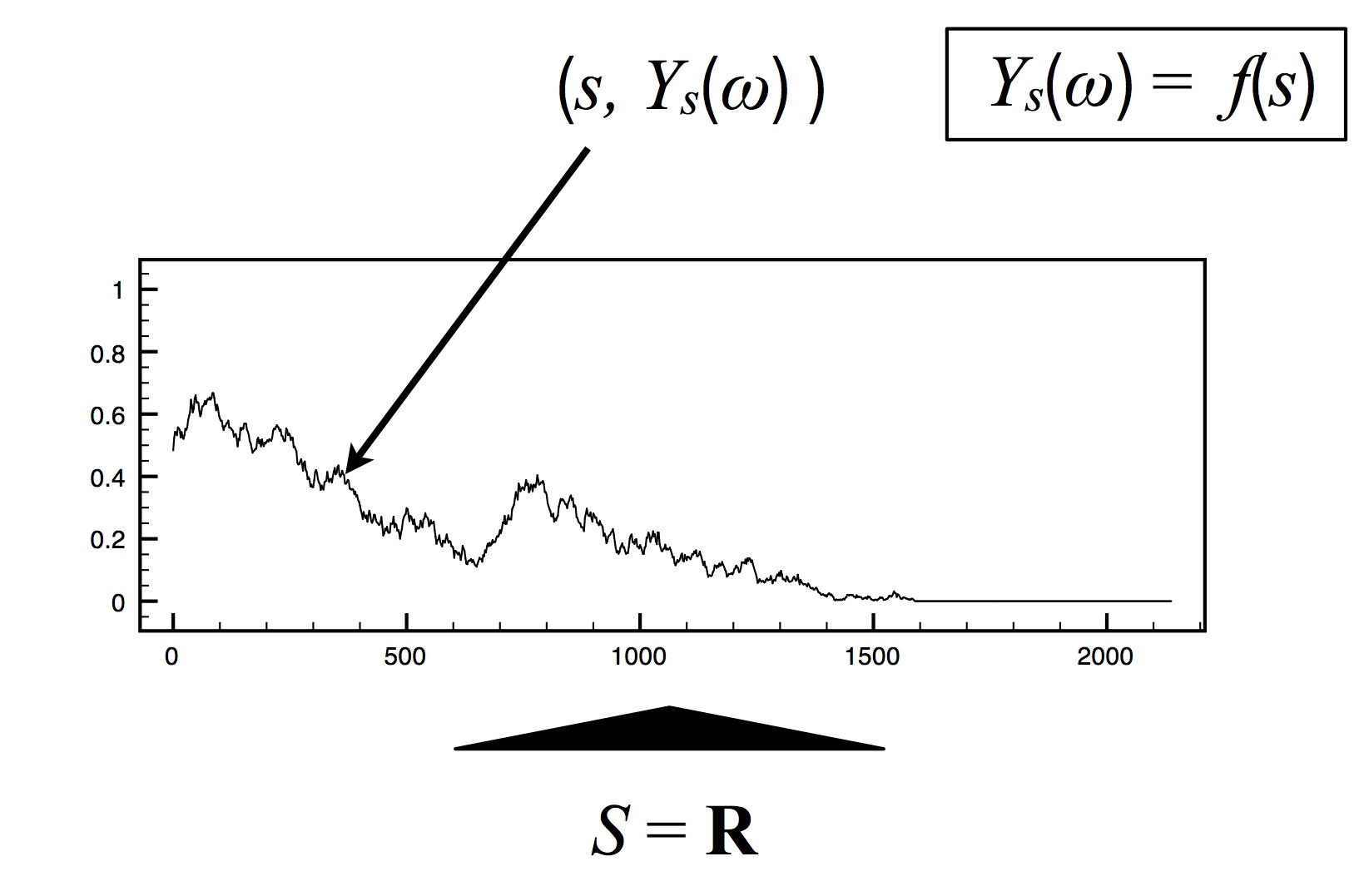

• $Y_s(\omega) \in \RR$: value of the random variable with index $s\in S$. The variable $\omega$ denotes an outcome.
• Example: Brownian motion - Brownian motion is a sample path of a diffusion process models the trajectory of a particle embedded in a flowing fluid and subjected to random displacements due to collisions with molecules, which is called Brownian motion.
• Alternative view: random function. (Terminology: Path space of a stochastic process.)
• flexible classes of diffusions and jump processes -jump process has discrete movements rather than continuous- (we should be able to cover a bit of both in this course)
  • Continuous-time Markov chains (a mathematical model which takes values in some finite or countable set and for which the time spent in each state takes non-negative real values and has an exponential distribution),
  • stochastic PDEs (essentially partial differential equations that have random forcing terms and coefficients).
• Applications:
  • economic/financial indicators,
  • frequency of a population having a certain genetic mutation,
  • periodic phenomena: climate, crop statistics, etc.

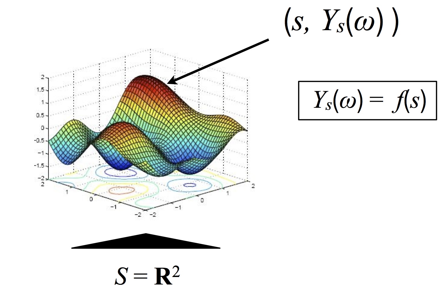
Natural generalizations:

• $S = \RR^2$: many applications in spatial statistics. $s=(longitude, latitude)$ and $Y_s$= concentration of a chemical at that location.
• $S = $ a space with a nice inner product structure (Hilbert space). Example we will cover: Gaussian processes.

Less natural but very useful: random measures: $S = \sa$, a sigma-algebra.

• Recall: a measure is a function that takes a set and returns a non-negative number, subject to countable additivity of disjoint sets constraints. (Countable additivity (or $\sigma$ additivity): The measure of the union of a finite number or an infinite countable number of sets that are pairwise disjoint is the sum of the measures of the sets.)
• Examples: Dirichlet process, Pitman-Yor process.
• Applications: mixture models (see below).
• Special case: point processes (integer-valued measure, the number of points that fall in a given set).

Motivation

We always have finite observations, why do we need uncountable spaces?

• We may not know yet where predictions will be needed.
• Theory predicts that we may be forced to use stochastic processes as latent variables: de Finetti theorem.

Terminology: Finite Dimensional Distributions (FDD)

More detailed overview via Forward Simulation

Forward simulation: generating a realization (or FDDs of a realization) of a stochastic process from scratch (without conditioning on any event). Synonym: generating a synthetic dataset. In contrast to:

Posterior simulation: obtain samples from the posterior distribution conditioning on some observed parts of the process.

Typically, forward simulation is much, much easier. This gives us another motivation for using stochastic processes: even when the inference method is very complicated and cannot be explained to non-experts, it is relatively simple to explain the model using forward simulation.

A simple jump process: a continuous-time Markov chain (CTMC)

Definition: A CTMC $Y_t(\omega)\in\Yscr, t\in\RR$ is specified by:

1. $\Yscr$, a finite set (the state space, not to be confused with $S$),
2. a transition probability matrix $M(y, y')$ over $\Yscr$ (we will interpret it as a jump probability, so let's assume there are no self transitions, $M(y,y) = 0$);
3. a positive number $\lambda_y$ associated to each state $y$, called a rate;
4. a starting point $y_0$.

To do forward simulation of a CTMC, do the following:

1. Initialize $y = y_0$, $p = ()$ to an empty list.
2. Repeat:
   1. Simulate a waiting time: use an exponential distribution with the rate corresponding to the current state, $\Delta t \sim \Exp(\lambda_y)$.
   2. Add a new segment to the piecewise constant path: $p \gets p \circ (y, \Delta t)$, where $\circ$ denotes concatenation (i.e. we represent a path with a list of pair, where each pair has the length of a segment, $\Delta t$, and its state $y$).
   3. Simulate a transition: use a categorical distribution with the probabilities given by row $y$ of the transition matrix, $y' \sim \Cat(M(y,\cdot))$.
   4. Update the current state: $y \gets y'$

Note: you may have seen different definitions. They are equivalent. Sometimes the one above is more convenient (for forward simulation, for example), sometimes, other definition/representations are more convenient (for example, the rate matrix representation is more convenient for obtaining FDDs). This will be an important idea in this course, not just with CTMC but also with all the other processes.

Applications: change point detection ($t$ is time), segmentation ($t$ is a position on the genome), survival analysis (add an absorbing state $y_{\textrm{death}}$ with corresponding rate $\lambda = 0$), molecular biology $\Yscr = \{\textrm{A,C,G,T}\}$. We may also cover more advanced examples where $\Yscr$ is countably infinite (examples: strings, counts in birth-death processes, RNA folding dynamics, chemistry ($\Yscr =$ count of different molecules undergoing chemical reactions).

A simple diffusion: Brownian motion

Diffusion: a continuous time, continuous space stochastic process with continuous paths.

Important example: Brownian motion (also known as Wiener process).

Definition: A collection of random variables $Y_s(\omega)\in\RR, s\in\RR$ such that:

1. For all, $s,t \in \RR$, the increments are normally distributed: \begin{eqnarray} (Y_{s+t} - Y_s) \sim N(0,\sigma^2 t) \end{eqnarray}
2. For any two disjoint intervals, $(t_1, t_2]$ and $(t_3, t_4]$, the increments $(Y_{t_2} - Y_{t_1})$ and $(Y_{t_4} - Y_{t_3})$ are independent.
3. The process starts at zero ($Y_0 = 0$) and its paths are continuous functions of $s$.

Theoretical question: Why is this a valid definition? In other words, what guarantees existence and uniqueness? Answer: Kolmogorov consistency theorem.

Practical question: How to sample from a Brownian motion? Example: using Monte Carlo, approximate the probability that a Brownian motion crosses the line $y=+1$ at least once in the interval $[0, 1/2]$.

Important idea: Lazy computing. Often, the question we try to answer does not require the knowledge of all points $Y_s$ (or at least, can be approximated using a finite number of points). Only instantiate the value at those points $s_i$ that matter.

Note: we may not know a priori what points matter. For example, with the above question may want to dynamically refine the approximation in a region very close to the line $y = +1$.

Refining the Brownian motion FDDs: Let's say we have only sampled $Y_{0.1}$ and $Y_{0.3}$. We want to add a sample $Y_{0.2}$ after the fact. How can we do this?

• Note: it can be shown that by characterization 1-3 above, $(Y_{0.1}, Y_{0.2}, Y_{0.3})$ has to be Multivariate Normal.
• Mean: $(0,0,0)$.
• Covariance: say $0 < s < t$, we have: \begin{eqnarray} \Cov(Y_s, Y_t) & = & \E[Y_s Y_t] \\ & = & \E[Y_s (Y_t - Y_s + Y_s)] \\ & = & \E[(Y_s)^2] + \E[Y_s - Y_0] \E[Y_t - Y_s] \\ & = & \sigma^2 s + 0. \end{eqnarray}
• Therefore, we can sample from the conditional distribution, $Y_{0.2} | (Y_{0.1}, Y_{0.3})$, which is also Normal—see Rasmussen's book on Gaussian processes, available online here.

Supplementary references and notes

Under construction

1- http://en.wikipedia.org/wiki/Continuous-timeMarkovchain

2- http://en.wikipedia.org/wiki/Brownian_motion