Instructor: Alexandre Bouchard-Côté

Editor: Hao Luo

Announcements

Background:

• Exercise 3
  • Released
  • Due on the 5th
  • Encouraged to work in teams (but write your own code)
  • Office hour on Monday 4-5
• Note: lowest grade on exercises will be dropped

Projects:

• Teams of 2 encouraged
• Topic (feel free to contact me if you want to run your idea with me or get more ideas)
  • Significant extension of one of the exercises
  • Original work in stoch process applied to stat/Bayesian analysis/computational statistics with some preliminary results (extending or creating a new process for a dataset of your choice, proposing a samplers, etc)
  • Some examples related to Exercise 3...

Wrapping up computational statistics

Cases where exact inference is possible

In some specialized cases, it is possible to do much better than MCMC and SMC, and we can get the exact value of $Z$ in polynomial time. Even when the whole problem is intractable, it is sometimes possible and beneficial to use exact inference method within approximate ones, for example as a block sampling techniques.

Again, we will start by assuming a discrete latent space, but the ideas here extends to other settings.

Background: We assume we are given a measure, $\mu$, with a normalization constant, $Z=||\mu||$, that would naively take an exponential time to compute. We assume that this measure is decomposed into a factor graph:

• Circles are variables we need to sum over
• Squares are factors/potentials in a product decomposition
• There is an edge if a factor needs to know the value of the connected variable

A factor/potential is simply a positive function. As a simple illustration, we can decompose the measure, $\mu(x,y,z) = f_1(x,y)f_2(y,z)f_3(z)$, into the factor graph below.

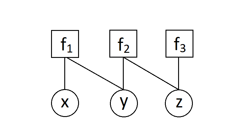
In the discrete case, this is implemented via a vector, matrix, or tensor.

Observations:

• This form of graph is related to directed graphical models, but with important differences. V structures in particular creates additional connections in factor graphs.
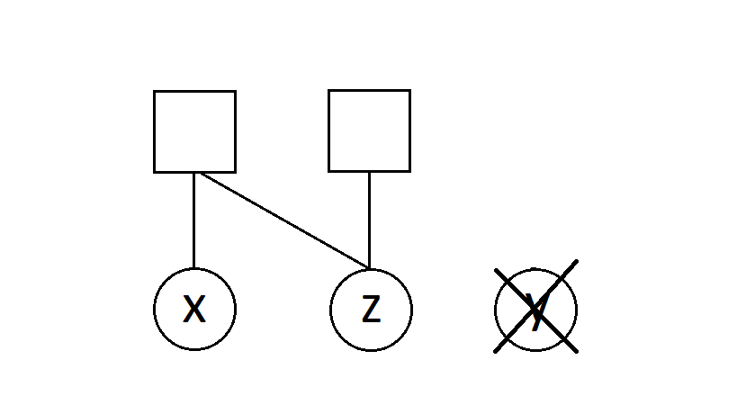
• We only need variables for the unobserved variables, as the value of the observed variable is fixed. For example, $\mu(x,y,z) = P(X=x, Z=z, Y=y)$ becomes $\mu(x,z) = P(X=x, Z=z, Y=y_0)$ after observing $Y=y_0$. The corresponding factor graph should only contain $x$ and $z$ as follows:

Computing the normalization of tree shaped factor graph:

• If we had a single node with a single variable, this is easy. With more than one variable, we can naively sum over all the variables but this is exponential.
• Instead, if we have bigger graphs, we just need to show that we can quickly perform two transformations such that:
  • One of the transforms produces a new factor graph $g'$ with one less factor than $g$, the other one produces a graph with one less variable.
  • Both transforms preserve the normalization, $\normof{g'} = \normof{g}$.

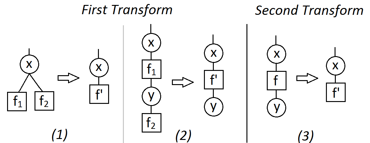
First transform: pointwise product. Removes two factors $f_1$ and $f_2$ and replace them by one new factor $f'$. Comes in two versions, depending on the arity of $f_2$ (number of connections):

\begin{eqnarray} f'(x) &=& f_1(x) f_2(x) \\ f'(x,y) &=& f_1(x) f_2(x,y). \end{eqnarray}

Second transform: marginalization. Removes one variable $x$ and replace a binary factor $f$ into a unary one $f'$.

\begin{eqnarray} f'(y) = \sum_x f(x,y). \end{eqnarray}

The figure below gives the graphical illustration of these transformations.

Remarks:

• If we have $N$ binary nodes, performing these two transformations can reduce the computational time from $2^N$ to $N \times 2 \times 2$.
• Except for the Gaussian case and some other very rare cases, the transformation generally does not work if the variable is continuous.

Optional exercises:

• Show that these two transforms preserve the normalization.
• Show that these two transforms can be used to change an arbitrary tree-shaped factor graph into a factor graph with a single variable and a single factor.
• Show how you can compute not only normalizations but also marginals over a single variable using the same algorithm. The only difference is that you will return the last factor, normalized.
• Show that you can modify the above algorithm to return all the one-node marginals by running the elimination along both directions of each edge.
• Show how you can modify this algorithms for the case where the potentials are multivariate normal distributions.

Point process

Background

Some factoids on Poisson processes we will need in this section

What is a Poisson process: In its full generality, a Poisson process (PP) is a distribution over countable multisets $S$ of points in a space $\Omega$ (multisets are sets where the points have multiplicities (counts)).

• A PP takes as a parameter a measure on $\Omega$ called the intensity measure $\mu$.
• A PP can also be viewed as random measure $M$ (where the measure of a set is the number of points that fall in it).
• Definition of a PP:
  • For all $A \subset \Omega$, $M(A) \sim \textrm{Poi}(\mu(A))$,
  • Disjoint sets should be assigned independent random masses: if $\{A_i\}$ is countable and disjoint, the random variables $\{M(A)\}$ should be independent.

Simulating from a Poisson process: Assume the space $\Omega$ has finite measure $\mu(\Omega)$, otherwise break it down into a partition with finite measure blocks (to support this, we assume that $\mu$ is $\sigma$-finite).

1. Sample the total number of points $N$ in the random multiset using a Poisson$(\mu(\Omega))$ random variable.
2. Normalize $\mu$ into $\bar \mu$.
3. Sample $N$ times from $\bar \mu$. Return these $N$ samples with their multiplicities.

Compound PP and Campbell theorem: If we have a PP $S$ on $\Omega$ with a finite intensity measure $\mu$, and a function $f : \Omega \to \RR$, a compound Poisson process construction is defined as the following random sum:

\begin{eqnarray} Y = \sum_{X \in S} f(X) \end{eqnarray}

Remarkably, it is possible to gain information on the distribution of this random sum via its characteristic function:

\begin{eqnarray} \E\left[ e^{itY} \right] = \exp\left\{ \int \left(e^{i t f(x)} - 1 \right) \mu(\ud x) \right\} \end{eqnarray}

Application 1: Creating a Bayesian non-parametric prior over unnormalized measures

Example:

• DP($H_0, \alpha_0$) was a prior over probability measures (where $H_0$ was mean or base measure parameter, say with density $p$).
• What if we need a prior over unnormalized measures? Example: non-parametric Cox process.
• Moran Gamma process: prior over unnormalized measures!
• Note: as in the DP, the MGP will have countable support with probability one.

Simplification: in our example, instead of random measures over $\Omega = \RR \times [0, \infty)$, let us just pick $\Omega = [0,1]$. This is just to make it easier to draw plots.

Consequence: we can draw two plots representing the random unnormalized measures:

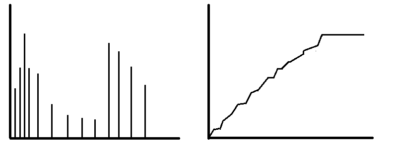
1. via a random probability measure mass functions (mmf), similar to the left panel of the figure to the right, and
2. via a random cumulative distribution functions, similar to the right panel of the figure to the right.

We will start by a Poisson-based way of simulating (1), then revisit (2) and formalize the Kolmogorov consistency axioms from earlier at the same time.

Using the Poisson to generate random mmf's:

1. If you want mmf on $\Omega$, sample PP on $\Omega \times [0, \infty)$. For example, $[0,1] \times [0, \infty)$ in our case.
2. Carefully design an intensity measure $\nu$ on $\Omega \times [0, \infty)$ (more on that later).
3. Interpret $x$-coordinate of each sampled point as a location, and the $y$-coordinate as the mass of that point.

Note: if you normalize these sticks, you get the Dirichlet process! But today we do not do this because we want a random unnormalized measure.

CDF view:

• Computing the cdf from the mmf is conceptually easy (but requires infinite amount of time).
• Let us say that for sake of interpretability we would like to have that the increments in the CDF between $t_1 < t_2$ be Gamma distributed, with:
  • shape parameter $H_0(t_2 - t_1)$ and
  • rate $\beta_0 = 1$.
• Can we carefully choose the intensity measure $\nu$ to satisfy this desiderata?

Yes!: check via Campbell theorem that if we pick $\nu$ (called a Levy measure in this context) with joint density:

\begin{eqnarray} y^{-1} e^{-y} p(x) \end{eqnarray}

where $p(x)$ is the density of $H_0$, then we get that jumps between $t_1 < t_2$ (sum $Y$ of sticks height $f(x,y) = y$ that fall in $[t_1, t_2]$) has characteristic function

\begin{eqnarray} \left( 1 - i t\right)^{-H_0([t_1, t_2])}, \end{eqnarray}

which is the characteristic function of a gamma random variable!

Note: this is an instance of a general recipe for constructing completely random measures (CRMs), which are the random measures where the mass of all disjoint sets are independent.

Kolmogorov consistency: We could have started differently, defining first a collection of FDDs $\nu_{t_1, t_2, \dots, t_K}$ over the heights of cdf at any finite locations $t_1, t_2, \dots, t_K$. If we denote the sorted locations by $t_{(1)}, t_{(2)}, \dots, t_{(K)}$, we would ask that the density of $\nu$ be given by:

\begin{eqnarray} n(h_1, \dots, h_K) = \gammarv(h_{(2)} - h_{(1)}; H_0[t_{(1)}, t_{(2)}], \beta_0) \times \dots \times \gammarv(h_{(K)} - h_{(K-1)}; H_0[t_{(K-1)}, t_{(K)}], \beta_0). \end{eqnarray}

Kolmogorov consistency states that there exists a process for which $\{\nu\}$ are the marginal iff the distributions $\nu$ satisfy:

1. Each $\nu$ is invariant under permutation (obvious here since the right-hand side is defined in terms of the ordered measure inputs).
2. The marginals are consistent under marginalization: for all $K$, we have:

\begin{eqnarray} \nu_{t_1, t_2, \dots, t_K}(A_1 \times \dots \times A_{K-1} \times \RR) = \nu_{t_1, t_2, \dots, t_{K-1}}(A_1 \times \dots \times A_{K-1}). \end{eqnarray}

This second condition can be checked with the properties of gamma random variable we discussed last time we talked about Kolmogorov consistency.

Application 2: Creating a Bayesian non-parametric prior over infinite latent features

Motivation: modelling customer choices via latent features.

Given a finite set of types of products (e.g. laptop, cellphone, etc.) and a finite number of choices for each, you ask people questions of the form 'you you buy an android or an iphone?'.

What we can do so far: cluster people, e.g. 'thrifty people' vs. 'extravagant'. Problem: one can imagine other useful clustering that are overlapping, e.g. 'people in their 0-19', '20-29', '30-39', '40+'. The problem is that we did not take note or have access to these (e.g. because of privacy). These are then called latent features.

Idea: instead of assigning each datapoint (person interviewed) exactly one $\theta$, let us assign them a set of thetas, $\{\theta\}$.

Given the $\{\theta\}$ we can easily build a parametric model over choices (e.g. with GLM machinery).

Matrix picture.

Beta process: Instead of an infinite list of sticks that sum to one, we want an infinite list of stick each between zero and one, but that do not need to sum to one. (can you see the difference with the gamma process?)

Then each customer flips a coin for each stick, with the bias given by the height of the stick. This specifies whether the customer picks the corresponding dish $\theta$. We want the probabilities to decay fast enough to guarantee that only a finite number of dishes are picked by each customer (but not too fast, so that the number of dishes used across all customers always grows).

It turns out it is possible to construct such random list by simply modifying the Levy measure into:

\begin{eqnarray} y^{-1} (1-y)^{c} p(x), \end{eqnarray}

where $c$ is a positive constant hyper-parameter.

With this choice, much of the machinery we have developed in the DP case can be also developed for this new process. See Miller 2011 for detail, here we will only cover the highlight:

Indian Buffet Process (IBP): an exchangeable distribution over the sampled sets $\underline{\{\theta_i\}}$, which is to the beta process what the CPR is to the DP:

1. The first customer picks a Poisson distributed number of dishes, with parameter $c$.
2. Customer $n+1$ does the following:
   • Look at each dish that was picked more than once before. For each one, if $i \ge 1$ is the number of times it has been taken before, take it as well independently with probability $i/(c+n)$.
   • Pick a Poisson distributed number of new dish, with rate parameter $c/n$.

Application 3: Other normalized completely random measures

Interestingly, the PY process cannot be constructed this way (by normalizing a CRM). However, other normalized CRMs offer interesting generalization to Dirichlet processes.

An important example is the Generalized Gamma CRM, with Levy measure given by:

\begin{eqnarray} \frac{a}{\Gamma(1-\sigma)} y^{-\sigma - 1} e^{-\tau y} p(x), \end{eqnarray}

where $a > 0$, $\sigma \in (0,1)$ and $\tau \ge 0$ are hyper-parameters.

See Favaro and Teh, 2013.

Note: Research project examples.

• Urban statistics and MGP.
• What happens if you multiply a Gamma r.v. with a PY?

What is next?

Here is an overview of some other active topics (each with a review/representative/recent paper) in the Bayesian non-parametric literature. We may spend more time on one or two of these, depending on the level of interest. Let me know if you think one of these will be particularly useful for your research.

• Infinite Hidden Markov Models: A stick breaking process gives us prior over a generalized multinomial. Now, imagine we view each of these as the row of a matrix and we generate an infinite list of rows (via a HDP). What do we get?
• Dependent Dirichlet Processes: Suppose now that we want a transient process. We can do this for example by introducing new sticks over time.
• Indian Buffet Process: So far, we have assumed that each customer picks a single table/parameter. It is sometimes useful for each customer to be able to pick a random set of parameters instead.
• Normalized Random Measures: Just as PY processes generalize DP, NRMs provide another route for generalizing DPs, with new efficient samplers being developed.
• Gamma-exponential process: A prior over infinite rate matrices.
• Fragmentation-Coagulation
• Random graphs

Supplementary references and notes

Under construction