Instructor: Alexandre Bouchard-Côté

Editor: Neil Spencer

TODO: Office hours scheduling

Theoretical properties of DPs (continued)

Summary of material from last time

FDDs of a process:

• Finite Dimensional Distribution
• In the case of a random measure: the measure evaluated at each of the blocks in a partition.

Kolmogorov definition/characterization of DPs: a random measure is a Dirichlet process iff the FDDs are Dirichlet distributions ($\star$)

Conjugacy: of DP $G$ and (generalized) multinomial sampling $\utheta | G$ (i.e., $G|\utheta$ is a DP with updated hyperparameters).

Why this is true:

• FDDs are Dirichlet distributions (by $(\Rightarrow)$ of ($\star$))
• Therefore, FDDs of $G|\utheta$ are Dirichlet distributions
• Therefore, $G|\utheta$ is a Dirichlet process (by $(\Leftarrow)$ of ($\star$))

CRP follows from the same argument: via the predictive distribution of a Dirichlet-multinomial model.

Moments of a DP

In this section, we derive the first and second moments of $G(A)$, for:

• $G \sim \dirp(\alpha_0, G_0)$ and
  
• $A \subset \Omega$ (fixed, deterministic).
  

To do this derivation, we use the Kolmogorov definition and consider the partition $(A, A^c)$ of $\Omega$.

We get: \begin{eqnarray} (G(A), G(A^c)) \sim \mbox{Dir}(\alpha_0G_0(A), \alpha_0G_0(A^c)). \end{eqnarray} This implies that: \begin{eqnarray} G(A) \sim \mbox{Beta}(x, y), \end{eqnarray} where $x$ denotes $\alpha_0G_0(A)$, and $y$ denotes $\alpha_0G_0(A^c)$.

The first moment: of $G(A)$ is therefore: \begin{eqnarray} \E[G(A)]=\frac{x}{x+y}=\frac{\alpha_0G_0(A)}{\alpha_0G_0(A)+\alpha_0G_0(A^c)}=G_0(A), \end{eqnarray} and the second moment of $G(A)$ is \begin{eqnarray} \var[G(A)] &=& \frac{xy}{(x+y)^2(1+x+y)} \\ &=&\frac{\alpha_0^2G_0(A)(1-G_0(A))}{\alpha_0^2(\alpha_0+1)} \\ &=&\frac{G_0(A)(1-G_0(A))}{\alpha_0+1}. \end{eqnarray}

This gives an interpretation of $\alpha_0$ as a precision parameter for the Dirichlet process.

Inference using DPMs (Dirichlet Process Mixture model): an end-to-end example

Goals of this section:

• show the detail of using a DP to answer a statistical question.
• We will introduce along the way two MCMC techniques that can be used to approximate the posterior.
  
• We will also look at the question of how to use the posterior to answer the task at hand.

Statistical tasks considered:

• Density estimation: The task in density estimation is to give an estimate, based on observed data, of an unobservable underlying probability density function. The unobservable density function is thought of as the density according to which a large population is distributed; the data are usually thought of as a random sample from that population.
  
• Clustering: In cases where the population is thought as being the union of sub-populations, the task of cluster analysis is to find the sub-population structure (usually without labeled data). Let us assume for simplicity that we wish to separate the data into two clusters. _{Note that the Dirichlet process is still a useful tool, even when the number of desired cluster is fixed. This is because each cluster that is output may need internally more than one mixture to be explained adequately under the likelihood model at hand. Note also that the DPM is not necessarily the right tool for finding a point estimate on the number of cluster components, in contrast to popular belief: see Miller and Harrison, 2013 for a simple cautionary example of inconsistency of the DPM for identifying the number of components.}

Bayesian approach: Let us take a Bayesian approach to these problems. This means that we need to pick:

• A joint probability distribution over knowns and unknowns (prior+likelihood): we will pick the DPM as defined last week.
• A loss function: let us look at a detailed example.

Examples of loss functions

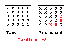
In the case of clustering, a popular choice is the rand loss between a true and putative labeled partitions $\rhot, \rhop$, denoted by $\randindex(\rhot, \rhop)$._{Note that we turn the standard notion of rand index into a loss by taking 1 - the rand index.}

---

Definition: The rand loss is defined as the number of (unordered) pairs of data points indices ${i,j}$ such that $(i \sim_{\rhot} j) \neq (i \sim_{\rhop} j)$, i.e.: \begin{eqnarray} \sum_{1\le i < j \le n} \1[(i \sim_\rhot j) \neq (i \sim_\rhop j)], \end{eqnarray} where $(i \sim_\rho j) = 1$ if there is a $B\in\rho$ s.t. $\{i,j\}\subseteq B$, and $(i \sim_\rho j) = 0$ otherwise.

In other words, a loss of one is incurred each time either: (1) two points are assumed to be in the same cluster when they should not, or (2) two points are assumed to be in different clusters when they should be in the same cluster.

---

The rand loss has several problems, motivating other clustering losses such as the adjusted rand index, but we will look at the rand loss here since the derivation of the Bayes estimator is easy for that particular loss. (See Fritsch and Ickstadt, 2009 for discussion on other losses and how to approach the Bayes estimator optimization problem for these other losses.)

In the case of density estimation, if the task is to reconstruct the density itself, examples of loss functions include the Hellinger and KL losses. However, density estimation is usually an intermediate step for another task, and the loss should then be defined on this final task rather than on the intermediate density estimation task.

Combining probability models and loss functions to do inference

Warning: in this lecture, we use a slightly different notation for the cluster indicators and observations of a DP. We make this change to avoid using the letter $Z$ for random variables, as it is often use in the sampling literature as a normalization constant.

• We now use the random vector $X$ to represent the cluster indicators.
• We now use the random vector $Y$ to represent the observations.
  

As reviewed earlier, the Bayesian framework is reductionist: given a loss function $L$ and a probability model $(X, Y) \sim \P$, it prescribes the following estimator: \begin{eqnarray} \argmin_{x} \E[L(x, X) | Y]. \end{eqnarray}

We will now see with the current example how this abstract quantity can be computed or approximated in practice.

First, for the rand loss, we can write: \begin{eqnarray} \argmin_{\textrm{partition }\rho} \E\left[\randindex(X, \rho)|Y\right] & = & \argmin_{\textrm{partition }\rho} \sum_{i<j} \E \left[\1 \left[\1[X_i = X_j] \neq \rho_{ij}\right]|Y\right] \\ &=&\argmin_{\textrm{partition }\rho} \sum_{i<j} \left\{(1-\rho_{ij})\P(X_i= X_j|Y) + \rho_{ij} \left(1- \P(X_i = X_j |y)\right)\right\} \label{eq:loss-id} \end{eqnarray} where $\rho_{i,j} = (i \sim_{\rho} j)$.

The above identity comes from the fact that $\rho_{i,j}$ is either one or zero, so:

• the first term in the the brackets of Equation~(\ref{eq:loss-id}) corresponds to the edges not in the partition $\rho$ (for which we are penalized if the posterior probability of the edge is large), and
• the second term in the same brackets corresponds to the edges in the partition $\rho$ (for which we are penalized if the posterior probability of the edge is small).

This means that computing an optimal bipartition of the data into two clusters can be done in two steps:

1. Simulating a Markov chain, and use the samples to estimate $\partstrength_{i,j} = \P(X_i = X_j | Y)$ via Monte Carlo averages.
2. Minimize the linear objective function $\sum_{i<j} \left\{(1-\rho_{ij})\partstrength_{i,j} + \rho_{ij} \left(1- \partstrength_{i,j}\right)\right\}$ over bipartitions $\rho$.

Note that the second step can be efficiently computed using min-flow/max-cut algorithms (understanding how this algorithm works is outside of the scope of this lecture, but if you are curious, see CLRS, chapter 26).

Our focus will be on computing the first step, i.e. the posterior over the random cluster membership variables $x_i$. Note that the $\partstrength_{i,j}$ are easy to compute from samples since the Monte carlo average of a function $f$ applied to MCMC samples converges to the expectation of the function under the stationary distribution (as long as $f$ is integrable, which is the case here since the indicator function is bounded). Sampling will be the topic of the next section.

Sampling via the collapsed representation

At each iteration, the collapsed sampler maintains values only for the cluster membership variables $x$, or more precisely, a labeled partition $\rho$ over the datapoints, which, as we saw last time, is sufficient thanks the Chinese Restaurant Process representation.

Recall: we write $(\rho(X) = \rho)$ for the labeled partition induced by the cluster membership variables (overloading $\rho(\cdot)$ to denote also the function that extracts the labeled partition induced by the cluster membership variables).

Note that ideally, we would like to know, for each $\rho$, the exact value of the posterior distribution: \begin{eqnarray}\label{eq:exact} \pi(\rho) = \P(\rho(X) = \rho | Y = y) = \frac{\P(\rho(X) = \rho, Y = y)}{\P(Y = y)}. \end{eqnarray} We have shown last week that we can compute the numerator for each partition $\rho$, via the following formula: \begin{eqnarray} \P(\part(X) = \part, Y = y) & = & \CRP(\part; \alpha_0) \left( \prod_{B \in \part} m(y_B) \right). \end{eqnarray}

The problem comes for the denominator, which involves summing over all partitions of the data: \begin{eqnarray} Z = \P(Y = y) = \sum_{\textrm{part} \rho'} \P(\rho(X) = \rho', Y = y). \end{eqnarray}

This is why we resort to an approximation of Equation~(\ref{eq:exact}). We show in detail how this problem can be approached via MCMC, removing the need to compute $Z$. MCMC only requires evaluation of the target density $\pi$ up to normalization, a quantity we call $\tilde \pi$ (the numerator of Equation~(\ref{eq:exact})).

---

Quick review of MCMC: (if you feel rusty on this, you should still be able to follow today, but come to office hour this week for a refresher).

• General idea: construct a Markov chain with stationary distribution $\pi$.
• The states visited (with multiplicities) provide a consistent approximation of posterior expectations via the law of large number for Markov chains.
• Start with a proposal $q$, transform it into a transition $T$ that satisfies detailed balance $\pi(x) T(x \to x') = \pi(x') T(x' \to x)$ (which implies $\pi$-invariance) by increasing the self-transition probability (rejection).
• Concretely, accept a state $x'$ proposed from $x$ with probability given by the Metropolis-Hastings ratio: \begin{eqnarray}\label{eq:mh} \min\left\{ 1, \frac{\pi(x')}{\pi(x)} \frac{q(x' \to x)}{q(x \to x')} \right\} = \min\left\{ 1, \frac{\tilde \pi(x')}{\tilde \pi(x)} \frac{q(x' \to x)}{q(x \to x')} \right\} \end{eqnarray}Importantly, note that the right-hand side sidesteps the difficulty of computing the normalization $Z$.
• To obtain irreducibility, mix or alternate transitions $T^{(i)}$ obtained from a collection of proposals $q^{(i)}$.

---

In the DPM collapsed Gibbs sampler, there will be one proposal $q^{(i)}$, each corresponding to a customer (datapoint). Each is a Gibbs move: this means that $q$ is proportional to $\pi$, but with a severely restricted support.

In our setup, the support is that we only allow one customer $i$ to change table when we are using proposal $q^{(i)}$.

Let us denote the partitions that are neighbors to the current state $\rho$ by $\rho'_1, \dots, \rho'_K$. By neighbor, we mean the states that can be reached by changing only the seating of customer $i$.

The Gibbs move simply consists in picking one of the neighbor or outcome $\rho'_k$ proportionally to the density of the joint: \begin{eqnarray}\label{eq:naive-way} p_k = \crp(\rho'_k; \alpha_0) \prod_{B\in \rho'_k} m(y_B). \end{eqnarray}

Some observations:

• Since $K-1$ is the number of tables after removing customer $i$, it is computationally feasible to sample from a multinomial over these $K$ outcomes. In particular, we can easily normalize $p_1, \dots, p_K$.
• An important property of Gibbs proposals is that they are never rejected (the acceptance ratio is one). This comes from the fact that $q$ is proportional to $\pi$, creating cancellations in Equation~(\ref{eq:mh}).
• While naively each move would take a running time $O(K^2)$ to perform (because each $p_k$ involves a product over $O(K)$ tables), this running time can be reduced to $O(K)$. This will be covered in the next exercise. Hint: the $p_k$s are also proportional (and in fact, equal) to the CRP predictive distributions.

Another DPM posterior sampling method

While the collapsed sampler is simple to implement and marginalizes several random variables, this sampler is harder to parallelize and distribute (why?), a major concern when scaling DPMs to large datasets.

The stick breaking representation gives an alternative way to sample that is more amenable to parallelization. It also gives an easy framework to approach non-conjugate models.

To avoid truncation, we will extend the idea you used for stick-breaking forward simulation (exercise 1, question 2). This will be done using auxiliary variables.

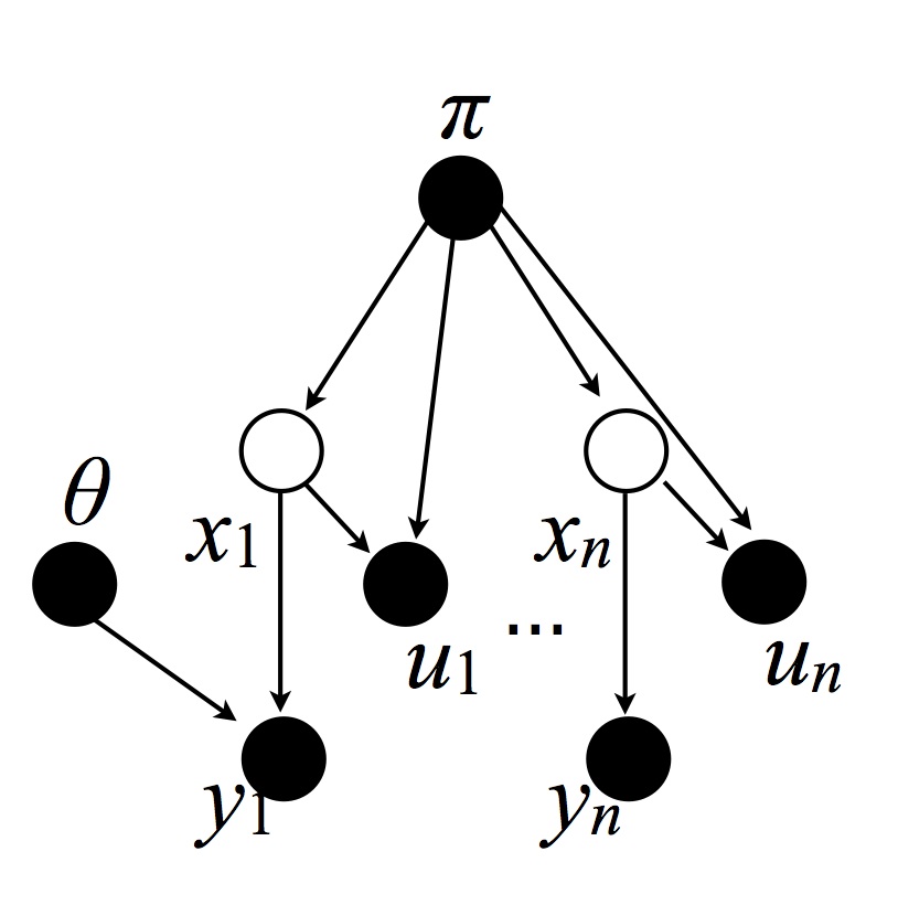
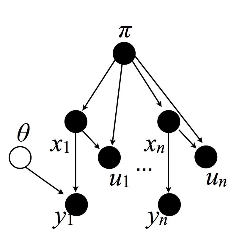
We first introduce some auxiliary variables $U$, more precisely one for each datapoint:

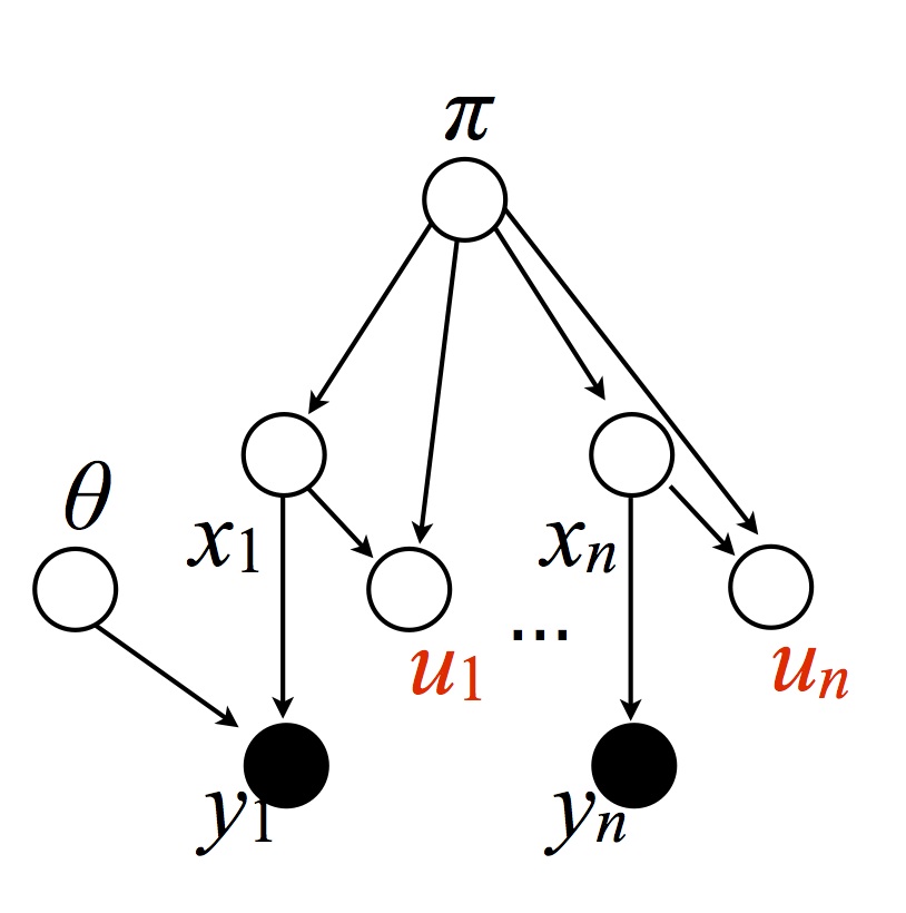
Warning: there is a missing edge between $\theta$ and $y_n$. Similarly for subsequent figures.

where $U_i|(X_i, \pi) \sim \textrm{Uni}(0, \pi_{X_i})$. _{Note: $\pi$ is used here as the distribution induced by stick, while in the previous section it $\pi$ was used as the target distribution. Since the two are of different types, this will not create ambiguities.} This yields the following joint probability (imagine an integral on both sides to interpret the $\ud \theta$, etc): \begin{eqnarray}\label{eq:joint-auxv} \P(\ud \theta, \ud \pi, X = x, \ud y, \ud u) &=& G_0^\infty(\ud \theta) \gem(\ud \pi; \alpha_0) \P(X = x|\pi) \prod_{i=1}^n \ell(\ud y_i | \theta_{x_i}) \unif(\ud u_i; 0, \pi_{x_i}). \\ &=& G_0^\infty(\ud \theta) \gem(\ud\pi; \alpha_0) \prod_{i=1}^n \1[0 \leq u_i \leq \pi_{x_i}] \ud u_i \ell(dy_i|\theta_{x_i}) \end{eqnarray} where we used $\P(X_i = c|\pi) \unif(\ud u_i; 0, \pi_{x_i}) = \1[0 \leq u_i \leq \pi_{x_i}] \ud u_i$ by the definition of uniform distributions (a uniform on an interval of length $b$ has a normalization of $b$) and $\P(X_i = c |\pi) = \pi_c$, also by definition.

The slice sampler proceeds by resampling the variables in three blocks: (1) all the dishes $\theta$, (2) all the cluster membership variables, and (3), both all the stick lengths and all the auxiliary variables.

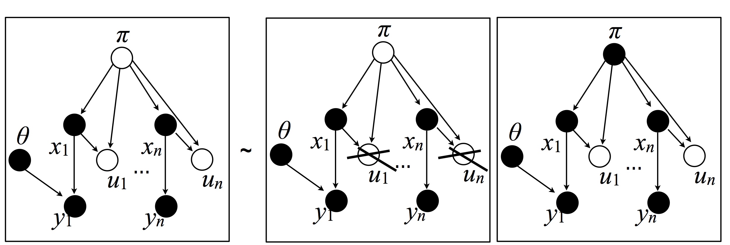
Cluster membership variables: This move resamples the following variables:

This can be done by resampling each one independently (conditionally on the Markov blanket; this follows from Bayes Ball).

To find the conditional distribution of $X_i = c$, for each $c=1, 2, \dots$, we look at the factors in Equation~(\ref{eq:joint-auxv}) that depend on $x_i$, and obtain: \begin{eqnarray} \P(X_i = c| \textrm{rest}) \propto \1[0 \le u_i \le \pi_c] \ell(\ud y_i|\theta_c) \end{eqnarray}

Thanks to lazy computation, we do not have to instantiate an infinite list of $\pi_c$ in order to compute this. Instead, we find the smallest $N \in \ZZ^{+}$, such that $\sum_{c=1}^{N} \pi_c > 1- u_i$. For $c>N$, $\sum_{c=1}^{N} \pi_c > 1- u_i$, so $\1[0 \leq u_i \leq \pi_c]=0$.

Dishes: This move resamples the following variables:

Again, this can be done by resampling each $\theta_c$ independently (conditionally on the Markov blanket).

The posterior distribution of $\theta_c|\textrm{rest}$ is \begin{eqnarray} \P(\ud \theta_c| \textrm{rest}) \propto G_0(\ud\theta_c) \prod_{i: x_i=c} \ell(\ud y_i|\theta_c), \end{eqnarray} which can be resampled by Gibbs sampling in some conjugate models, and can be resampled using a Metropolis-Hastings step more generally.

Auxiliary variables and stick lengths: This resamples both all the auxiliary variables and all the stick lengths in one step. Using the chain rule, this step is subdivided in two substeps:

In other words: \begin{eqnarray} \P\left(\ud \pi, \ud u \big| \textrm{rest}\right) =& \P\left(\ud \pi\big| \textrm{ rest except for } u \right) \P\left(\ud u | \textrm{rest} \right)\ \end{eqnarray}

The second factor can be sampled from readily: \begin{eqnarray} \P(\ud u_i | \textrm{rest}) =& \unif(\ud u_i; 0, \pi_{x_i}). \end{eqnarray}

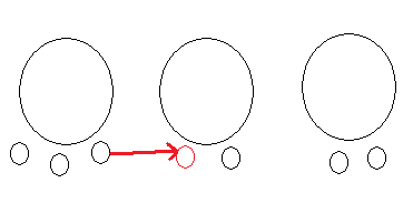
To sample from the first factor, we look at an equivalent, sequential decision scheme for sampling sticks that is an alternative to dart throwing. This sequential scheme makes it easier to see how to resample $\pi$ while integrating out the auxiliary variables.

This alternative consists in visiting the sticks in order, and flipping a coin each time to determine if we are going to pick the current stick, or a stick of larger index:

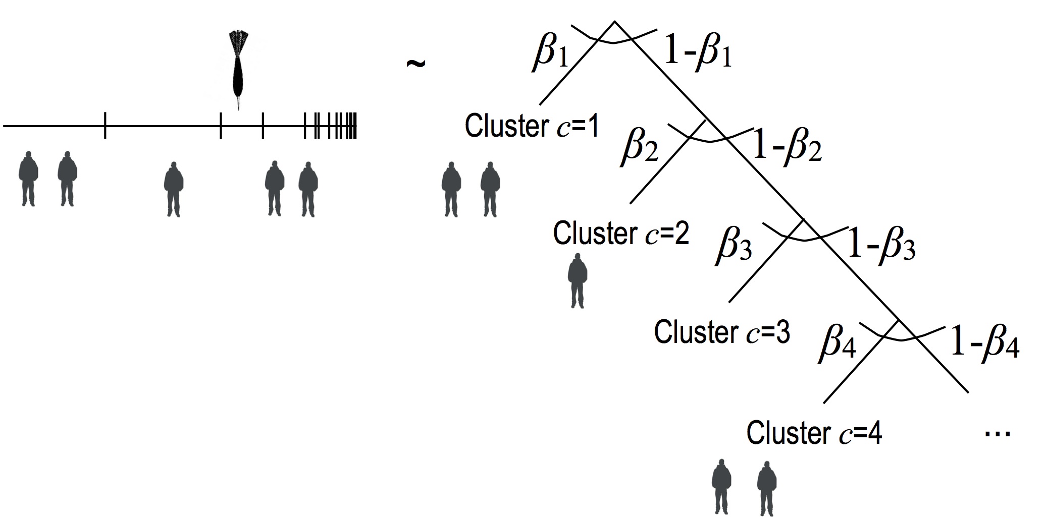
Here the persons represent datapoints, and the right-hand-side represents a decision tree. Since the $\beta_c \sim \betarv(1, \alpha_0)$, and that each decision in the decision tree is multinomial, we get by multinomial-dirichlet conjugacy: \begin{eqnarray} \P(\ud \pi_c| \text{ rest except for } u) = \betarv(\ud \pi_i; a_c, b_c) \end{eqnarray} where: \begin{eqnarray} a_c &=& 1+ \sum_{i=1}^{n}\1[x_i=c] \\ b_c &=& \alpha_0 + \sum_{i=1}^m \1[x_i >c] \end{eqnarray}

Comparison

We conclude this section by summarizing the advantages and disadvantages of each methods:

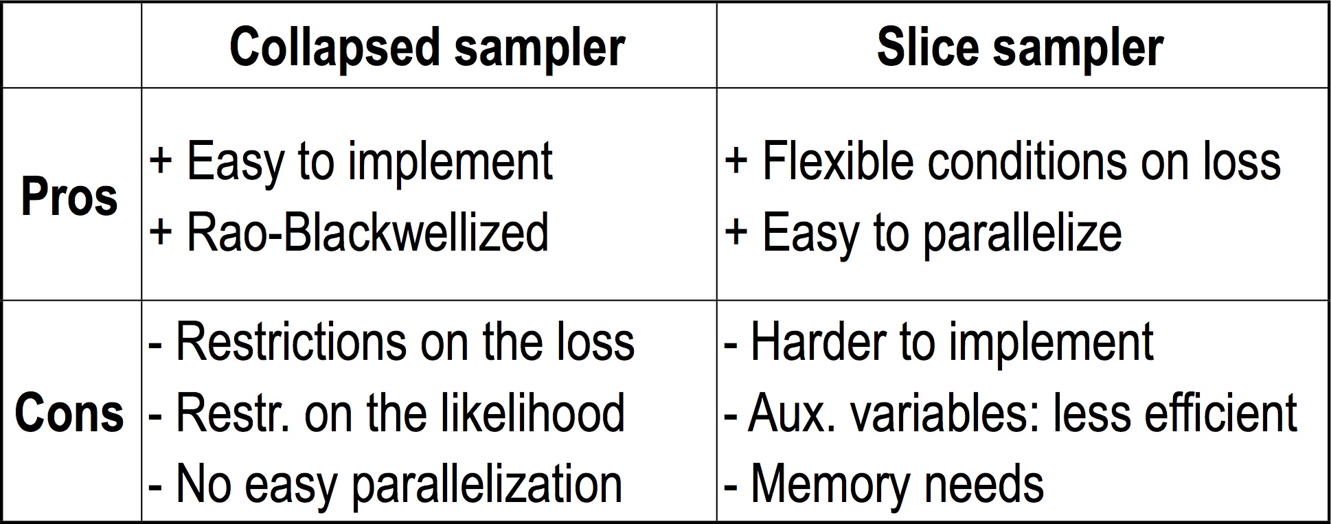
The restriction on the loss is that the expected loss needs to be computable from only samples from the cluster indicators. The restriction on the likelihood is the conjugacy assumption discussed in the section on the collapsed sampler. Note that Rao-Blackwellization does not necessarily mean that the collapsed sampler will be more efficient, since each sampler resamples different blocks of variables with a different computation cost per sample.

The memory needs of the slice sampler can get large in the case where the value of the auxiliary variables is low. Note that using a non-uniform distribution on the auxiliary variables could potentially alleviate this problem.

Note also that for some other prior distributions (for example general stick-breaking distributions, which are covered in the next set of notes), only the slice sampler may be applicable. In other extensions of the DP, both slice and collapsed samplers are available.

Supplementary references and notes

Porteous, I., Ihler, A. T., Smyth, P., & Welling, M. (2012). Gibbs sampling for (coupled) infinite mixture models in the stick breaking representation. arXiv preprint arXiv:1206.6845. Kalli, M., Griffin, J. E., & Walker, S. G. (2011). Slice sampling mixture models. Statistics and computing, 21(1), 93-105.