Instructor: Alexandre Bouchard-Côté

Editor: Jonathan Baik

More detailed overview via Forward Simulation (continued)

Recall: Forward simulation is the process of generating a realization (or FDDs of a realization) of a stochastic process from scratch (without conditioning on any event).

Synonym: generating a synthetic dataset. In contrast to:

Another synonym: generative process/story.

Random measures: motivation and Dirichlet process forward simulation

Based on lecture notes created the first time I taught this course: PDF.

Motivation: Mixture models.

Example: Modelling the weight of walruses. Observation: weights of specimens $x_1, x_2, ..., x_n$.

Inferential question: what is the most atypical weight among the samples?

Method 1:

• Find a normal density $\phi_{\mu, \sigma^2}$ that best fits the data.
• Bayesian way: treat the unknown quantity $\phi_{\mu, \sigma^2}$ as random.
• Equivalently: treat the parameters $\theta = (\mu, \sigma^2)$ as random, $(\sigma^2 > 0)$. Let us call the prior on this, $p(\theta)$ (for example, another normal times a gamma, but this will not be important in this first discussion).

Limitation: fails to model sexual dimorphism (e.g. male walruses are typically heavier than female walruses).

Solution: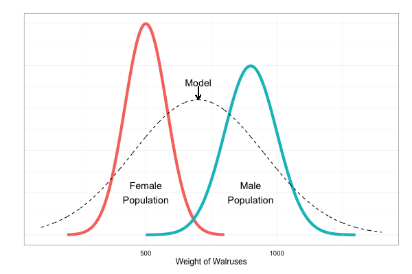

Method 2: Use a mixture model, with two mixture components, where each one assumed to be normal.

• In terms of density, this means our modelled density has the form: $$\begin{eqnarray} \phi = \pi \phi_{\theta_1} + (1 - \pi) \phi_{\theta_2}, \end{eqnarray}$$ for $\pi \in [0, 1]$.
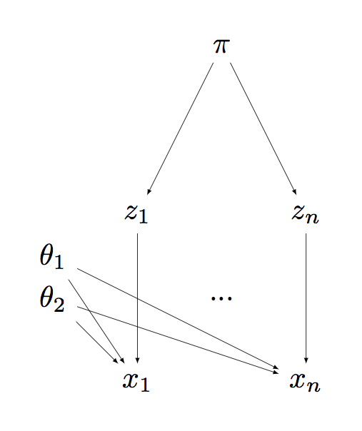
• Equivalently, we can write it in terms of auxiliary random variables $Z_i$, one of each associated to each measurement $X_i$: $$\begin{eqnarray} Z_i & \sim & \Cat(\pi) \\ X_i | Z_i, \theta_1, \theta_2 & \sim & \Norm(\theta_{Z_i}). \end{eqnarray}$$
• Each $Z_i$ can be interpreted as the sex of animal $i$.

Unfortunately, we did not record the male/female information when we collected the data!

• Expensive fix: Do the survey again, collecting the male/female information
• Cheaper fix: Let the model guess, for each data point, from which cluster (group, mixture component) it comes from.

Since the $Z_i$ are unknown, we need to model a new parameter $\pi$. Equivalently, two numbers $\pi_1, \pi_2$ with the constraint that they should be nonnegative and sum to one. We can interpret these parameters as the population frequency of each sex. We need to introduce a prior on these unknown quantities.

• Simplest choice: $\pi \sim \Uni(0,1)$. But this fails to model our prior belief that male and female frequencies should be close to $50:50$.
• To encourage this, pick a prior density proportional to: $$\begin{eqnarray} p(\pi_1, \pi_2) \propto \pi_1^{\alpha_1 - 1} \pi_2^{\alpha_2 - 1}, \end{eqnarray}$$
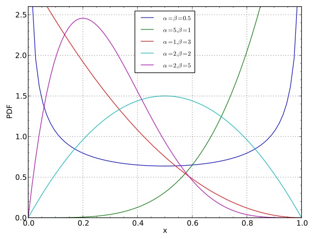
  where $\alpha_1 > 0, \alpha_2 > 0$ are fixed numbers (called hyper-parameters). The $-1$'s give us a simpler restrictions on the hyper-parameters required to ensure finite normalization of the above expression).
• The hyper-parameters are sometimes denoted $\alpha = \alpha_1$ and $\beta = \alpha_2$.
  • To encourage values of $\pi$ close to $1/2$, pick $\alpha = \beta = 2$.
  • To encourage this even more strongly, pick $\alpha = \beta = 20$. (and vice versa, one can take value close to zero to encourage realizations with one point mass larger than the other.)
  • To encourage a ratio $r$ different that $1/2$, make $\alpha$ and $\beta$ grow at different rates, with $\alpha/(\alpha+\beta) = r$. But in order to be able to build a bridge between Dirichlet distribution and Dirichlet processes, we will ask that $\alpha = \beta$ _{(Comment that should be ignored in first reading: one way to obtain the DP from the Dirichlet, which we will not cover in this lecture, is as a weak limit of symmetric Dirichlet distributions, i.e. a generalization of the statement $\alpha = \beta$ (see wiki page). It may be interesting to ask what happens in the non-symmetric case. This may seem non-exchangeable a priori, but this is addressed when the atoms are sampled iid.).}

Dirichlet distribution: This generalizes to more than two mixture components easily. If there are $K$ components, the density of the Dirichlet distribution is proportional to: $$\begin{eqnarray} p(\pi_1, \dots, \pi_K) \propto \prod_{k=1}^{K} \pi_k^{\alpha_k - 1}, \end{eqnarray}$$ Note that the normalization of the Dirichlet distribution is analytically tractable using Gamma functions $\Gamma(\cdot)$ (a generalization of $n!$). See the wikipedia entry for details.

Important points:

• Each component $k\in \{1, \dots, K\}$ is associated with a probability $\pi_k$, and a value $\theta_k$.
• This is therefore a discrete measure with atoms at $(\theta_1, \dots, \theta_K)$ and probabilities given by the components of the vector $\pi = (\pi_1, \dots, \pi_k)$.

Formally:

• Let us say we are given a set $A \subset \RR \times (0, \infty)$
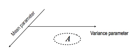
  • The space $\RR \times (0, \infty)$ comes from the fact that we want $\theta$ to have two components, a mean and a variance, where the latter has to be positive
  • Let us call this space $\Omega = \RR \times (0, \infty)$
• We can define the following probability mesure 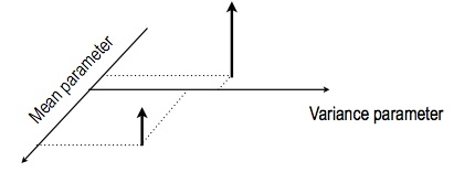$$\begin{eqnarray} G(A) = \sum_{k=1}^{K} \pi_k \1(\theta_k \in A), \end{eqnarray}$$ where the notation $\1(\textrm{some logical statement})$ denotes the indicator variable on the event that the boolean logical statement is true. In other words, $\1$ is a random variable that is equal to one if the input outcome satisfies the statement, and zero otherwise.

Random measure: Since the location of the atoms and their probabilities are random, we can say that $G$ is a random measure. The Dirichlet distribution, together with the prior $p(\theta)$, define the distribution of these random discrete distributions.

Connection to previous lecture: Another view of a random measure: a collection of real random variables indexed by sets in a sigma-algebra: $G_{A} = G(A)$, $A \in \sa$.

Limitation of our setup so far: we have to specify the number of components/atoms $K$. The Dirichlet process is also a distribution on atomic distributions, but where the number of atoms can be countably infinite.

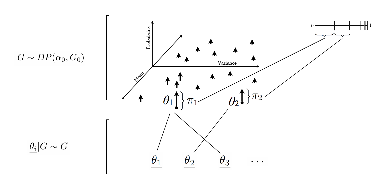
Definition: A Dirichlet process (DP), $G_A(\omega) \in [0, 1]$, $A \in \sa$, is specified by:

1. A base measure $G_0$ (this corresponds to the density $p(\theta)$ in the previous example).
2. A concentration parameter $\alpha_0$ (this plays the same role as $\alpha + \beta$ in the simpler Dirichlet distribution).

To do forward simulation of a DP, do the following: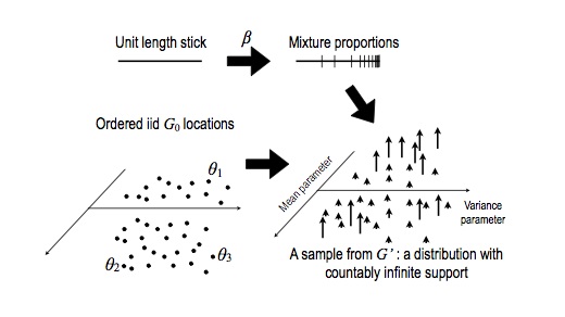

1. Start with a current stick length of one: $s = 1$
2. Initialize an empty list $r = ()$, which will contain atom-probability pairs.
3. Repeat, for $k = 1, 2, \dots$
   1. Generate a new independent beta random variable: $\beta \sim \Beta(1, \alpha_0)$.
   2. Create a new stick length: $\pi_k = s \times \beta$.
   3. Compute the remaining stick length: $s \gets s \times (1 - \beta)$
   4. Sample a new independent atom from the base distribution: $\theta_k \sim G_0$.
   5. Add the new atom and its probability to the result: $r \gets r \circ (\theta_k, \pi_k)$

Finally, return: $$\begin{eqnarray} G(A) = \sum_{k=1}^{\infty} \pi_k \1(\theta_k \in A), \end{eqnarray}$$

This is the Stick Breaking representation, and is not quite an algorithm as written above (it never terminates), but you will see in the first exercise how to transform it into a valid algorithm.

Sampling from a sampled measure

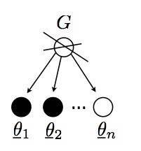
Since the realization of a DP is a probability distribution, we can sample from this realization! Let us call these samples from the DP sample $\underline{\theta_1}, \underline{\theta_2}, \dots$

$$\begin{eqnarray} G & \sim & \DP \\ \underline{\theta_i} | G & \sim & G \end{eqnarray}$$

Preliminary observation: If I sample twice from an atomic distribution, there is a positive probability that I get two identical copies of the same point (an atomic measure $\mu$ is one that assign a positive mass to a point, i.e. there is an $x$ such that $\mu(\{x\}) > 0$). This phenomenon does not occur with non-atomic distribution (with probability one).

The realizations from the random variables $\underline{\theta_i}$ live in the same space $\Omega$ as those from $\theta_i$, but $\underline{\theta}$ and $\theta$ have important differences:

• The list $\underline{\theta_1}, \underline{\theta_2}, \dots$ will have duplicates with probability one (why?), while the list $\theta_1, \theta_2, \dots$ generally does not contain duplicates (as long as $G_0$ is non-atomic, which we will assume today).
• Each value taken by a $\underline{\theta_i}$ corresponds to a value taken by a $\theta$, but not vice-versa.

To differentiate the two, I will use the following terminology:

• Type: the variables $\theta_i$
• Token: the variables $\underline{\theta_i}$

Question: How can we simulate four tokens, $\underline{\theta_1}, \dots, \underline{\theta_4}$?

1. Hard way: use the stick breaking representation to simulate all the types and their probabilities. This gives us a realization of the random probability measure $G$. Then, sample four times from $G$.
2. Easier way: sample $\underline{\theta_1}, \dots, \underline{\theta_4}$ from their marginal distribution directly. This is done via the Chinese Restaurant Process (CRP).

Let us look at this second method. Again, we will focus on the algorithmic picture, and cover the theory after you have implemented these algorithms.

The first idea is to break the marginal $(\underline{\theta_1}, \dots, \underline{\theta_4})$ into sequential decisions. This is done using the chain rule:

1. Sample $\underline{\theta_1}$, then,
2. Sample $\underline{\theta_2}|\underline{\theta_1}$,
3. etc.,
4. Until $\underline{\theta_4}|(\underline{\theta_1}, \underline{\theta_2}, \underline{\theta_3})$.

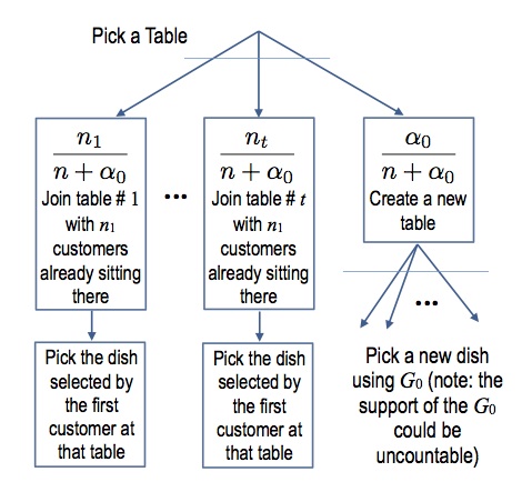
The first step is easy: just sample from $G_0$! For the other steps, we will need to keep track of token multiplicities. We organize the tokens $\underline{\theta_i}$ into groups, where two tokens are in the same group if and only if they picked the same type. Each group is called a table, the points in this group are called customers, and the value shared by each table is its dish.

Once we have these data structures, the conditional steps 2-4 can be sampled easily using the following decision diagram:

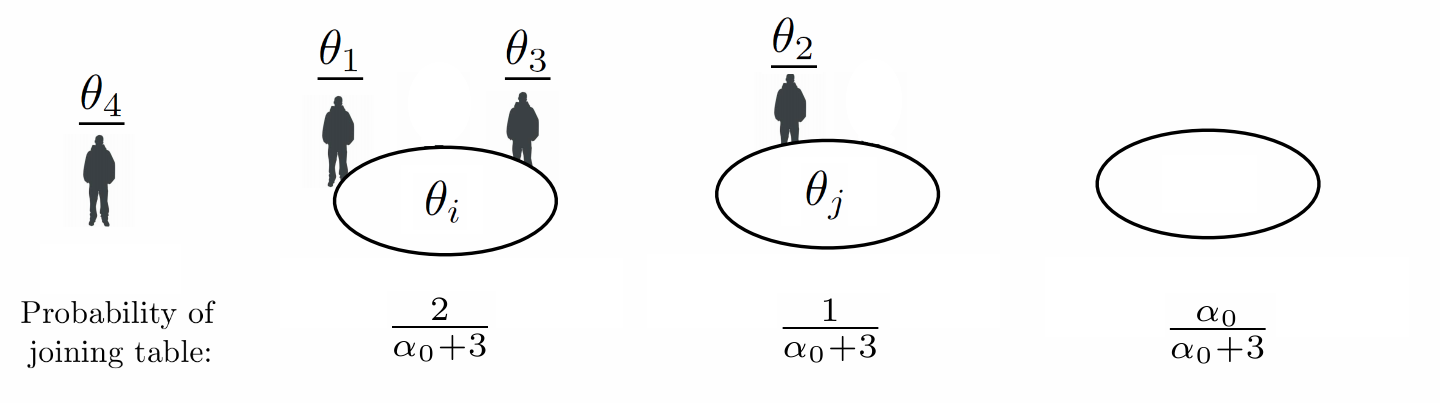
Following our example, say that the first 3 customers have been seated at 2 tables, with customers 1 and 3 at one table, and customer 2 at another. When customer 4 enters, the probability that the new customer joins one of the existing tables or creates an empty table can be visualized with the following diagram:

Formally:

$$\begin{eqnarray} \P(\underline{\theta_{n+1}} \in A | \underline{\theta_{1}}, \dots, \underline{\theta_{n}}) = \frac{\alpha_0}{\alpha_0 + n} G_0(A) + \frac{1}{\alpha_0 + n} \sum_{i = 1}^n \1(\underline{\theta_{i}} \in A). \end{eqnarray}$$

Clustering/partition view: This generative story suggests another way of simulating the tokens:

1. Generate a partition of the data points (each block is a cluster)
2. Once this is done, sample one dish for each table independently from $G_0$.

By a slight abuse of notation, we will also call and denote the distribution on the partition the CRP. It will be clear from the context if the input of the $\CRP$ is a partition or a product space $\Omega \times \dots \times \Omega$.

Important property: Exchangeability. We claim that for any permutation $\sigma : \{1, \dots, n\} \to \{1, \dots, n\}$, we have:

$$\begin{eqnarray} (\underline{\theta_1}, \dots, \underline{\theta_n}) \deq (\underline{\theta_{\sigma(1)}}, \dots, \underline{\theta_{\sigma(n)}}) \end{eqnarray}$$

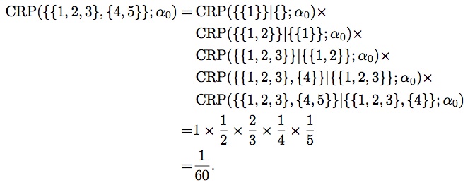
You will prove this property in the first exercise. In the meantime, you can convince yourself with the following small example, where we compute a joint probability of observing the partition $\{\{1,2,3\},\{4,5\}\}$ with two different orders. First, with the order $1 \to 2 \to 3 \to 4 \to 5$, and $\alpha_0 = 1$:

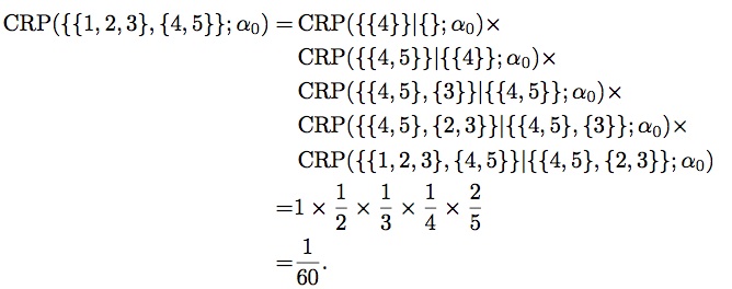
Then, with the order $4 \to 5 \to 3 \to 2 \to 1$, we get:

What's next?

Before going deeper into Bayesian non-parametrics, we will first review some important Bayesian concepts in the parametric setup. This will be the program for next week.

Supplementary references and notes

Teh, Y. W. (2010). Dirichlet processes. Encyclopedia of Machine Learning, 280-287. (Link to PDF)

Zhang, X. (2008). A Very Gentle Note on the Construction of Dirichlet Process. The Australian National University, Canberra. (Link to PDF)

Blackwell, D., & MacQueen, J. B. (1973). Ferguson distributions via Pólya urn schemes. The annals of statistics, 353-355. (Link to PDF)

Ferguson, T. S. (1973). A Bayesian analysis of some nonparametric problems. The annals of statistics, 209-230. (Link to PDF)

Sethuraman, J. (1994). A Constructive Definition of Dirichlet Priors. Statistica Sinica, 4, 639-650. (Link to PDF)

Neal, R. M. (2000). Markov chain sampling methods for Dirichlet process mixture models. Journal of computational and graphical statistics, 9(2), 249-265. (Link to PDF)